Cricket teams and the efficient frontier - Part 2

A while back I posted a largely ridiculous idea to create a financial market around cricket one-day international scores. In summary, the "stock" was a team's average score in ODIs throughout the year (with some assumptions, see the post). It was based around the idea that ODI scores have been increasing year-on-year since ODIs were invented. Using traditional financial market modelling techniques, we came up with an investment strategy for each of the teams, which involved mainly investing in South Africa and Bangladesh.

So, how did we go?

Unsurprisingly, not that well! Under the assumptions of the model, the average ODI score increased slightly from 266.8 to 267.5. So, if you had invested in the ODIAll index fund, you would have made a slight profit. If however you had chosen the market portfolio, you would have lost 14.4% of your money, largely on the back of diminished South African and Bangladeshi performances. Similarly, if you had not allowed short selling, you would have lost 9.8% of your money. And even the least risky minimum risk portfolio lost 4.8%.

Much like the real stock market, you best bet would have been to simply invest in the Index. Here is the updated risk/return chart.

If you are playing again in 2017, your strategy is similar to last year - perhaps reflecting that this method of measuring "stock performance" is not particularly good! Using a team's entire history to predict next year's scores is not the way I'd do it - you're better off looking at its recent history, who and where it is playing this year etc. I'd probably be investing in England in 2017. They seem to be finally learning how to play ODIs, although they had a very good 2016 so it would take an even better year to improve on that. And the Associates are getting better and better, with 3 set to join the 10 Test playing nations in a proper regular ODI league - they will be jostling for those positions so I expect performances to improve.

	Market Portfolio	No short selling	Minimum Risk Portfolio
Australia	-0.08	0.00	0.29
England	0.00	0.00	0.03
New Zealand	0.16	0.08	0.00
India	0.05	0.00	0.10
Pakistan	0.18	0.00	0.11
West Indies	-0.20	0.00	0.06
South Africa	0.40	0.23	0.20
Sri Lanka	-0.06	0.00	0.08
Zimbabwe	0.03	0.07	0.06
Bangladesh	0.44	0.58	0.07
Associate	0.08	0.05	0.00

Cricket teams and the efficient frontier

Cricket and financial markets have a rich, intertwined history, from Vincent back to Waugh/Warne, Lillee/Marsh and Keith Miller. So, I don't think we necessarily need a new cricket market, but let's make one anyway, and refresh my financial maths and linear algebra at the same time.

Cricket, especially its shortened forms, is seemingly becoming a batsman's game. Bats are bigger, fields are smaller, fielding and bowling restrictions make it difficult to pressure the batsmen, players are fitter and the game is more professional than it has ever been. The trend towards bigger scores is shown clearly in men's One-day International (ODI) cricket. The following chart shows the yearly average score each team scored when batting first in an ODI^*, with the black line (ODIAll) being the average of all games in that year. The "Associate" line refers to Associate cricket teams that played games the International Cricket Council (ICC) deemed worthy enough to have ODI status, and also those World XI, Asia XI and Africa XI matches that were in vogue about 10 years ago and were also given ODI status. Individual Associate nations did not play enough games to create enough meaningful data for this analysis.

ODI Scores
Create line charts

^*Only innings that went for 50-overs, or where the team was bowled out, were counted so as to take out the influence of rain.

In our financial market, each of the series above is a stock, whose value is that team's average ODI score batting first in that year. The ODIAll series is the index for this particular stock market (like the S&P 500 or All Ordinaries). The upward trend in ODIAll is clear, and the following shows ODIAll data with an exponential fit. An exponential fit is what you would expect if the stock was growing with continuously compounding interest. The fit is pretty good (R² = 0.8). The other dots are the country data and show the scatter (and noise) in the data set. I've gone back to 1980, as before then there were few games played annually.


Such trends are evident in other sports, but not all sports are as focused on increasing scores. Premier League football shows no such scoring trend, total home runs in Major League Baseball ebbs and flows depending on a number of factors including the amount of steroids being taken, but there has been a steady increase in strike outs over the last 20 years.

Let's do some maths. What we want to do is determine in which teams we should invest. We don't necessarily want to invest in the teams that regularly produce the highest scores. We want to pick the teams that are improving - that is, their stock prices are going up so we'll get a good return. For instance, Australia has been dominant in ODI cricket for some time; it may not be a good investment if it can not continue to grow its already large yearly average. On the other hand, Associate teams are playing more ODI cricket and Bangladesh is ever improving, perhaps they would be better investments, although likely to be more risky than an established team. Maybe we'd be better off just buying the ODIAll Index.

Inline with Modern Portfolio Theory, I used the methods in these two articles:

• Calculating the Efficient Frontier: Part 1  
• Portfolio optimization using the efficient frontier and capital market line in Excel

Yes, I did it in Excel, and yes I realise that if I was any sort of data analyst I would have done it in R, but if you can't go 80% of the way towards solving the problem in Excel, it's not a problem worth solving.

The following chart shows the average percentage return and standard deviation of each country's yearly stock price. On average, Australia increases its price by ~1%, with a standard deviation (risk) of 8%. Interestingly, South Africa, for a similar risk, has a ~2% return. Bangladesh is the BRIC of this market, rapidly improving over the last few years, but with a relatively high risk. The Associates are far too risky to invest in just yet. 
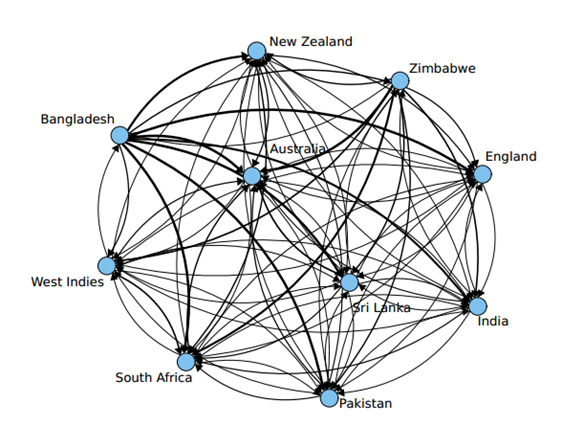
To determine your portfolio, you don't just need the risk/return values, but we also need to know whether an increase in one country's stock will cause an increase (or decrease) in another. This is measured by covariance. In our case, the prices of all countries are generally moving upwards over time, however there are some interesting pairs of countries that move together in the same direction (Sri Lanka and New Zealand) and in the opposite direction (Zimbabwe and Bangladesh). I suspect a lot of this is noise. In any case, by knowing that an increase in one stock price will likely see a decrease in another, you can minimise the overall risk of your portfolio by hedging.

To determine which teams we should include in our portfolio, we need to determine the Efficient Frontier. This is the line on which you can not get a higher return from any combination of assets in your portfolio for your choice of risk. For example, if you are happy to take on a risk of 20%, you can't expect a return more than 8% from these assets - yes, it's not exactly the sort of market I'd want to buy into, but let's keep going...

The next thing we need is the Capital Market Line (CML). In any market, there may be what is known as a "risk-free asset" - an asset which gives a guaranteed return with no risk. In financial modelling, government bonds assume the role of risk-free asset, as they have a known return and as the government has almost zero chance of default, are assumed risk-free. The CML is the line drawn from the point of the risk-free asset (on the y-axis) such that it is tangent to the efficient frontier. The intercept point is known as the market portfolio. Along the CML, your portfolio contains various amounts of the risk-free asset and the market portfolio (the risky asset).

There is no real equivalent to a risk-free asset in this market, so I've assumed it to be 0.5%, which is, at time of writing, about the price of a German 10-year government bond (this market is based in Germany, for no particularly good reason. Perhaps a German financier, tired of his team being ranked between Gibraltar and the Isle of Man, wanted some fun).

The market portfolio allows you to short sell; that is, sell stock you don't currently own. Perhaps you've borrowed it and sold it on. But you have to buy it back to give it back to the person from whom you borrowed it. You'd do this if you were expecting the price to drop so you would be buying it back at a lower price than you sold it, or as in our scenario, as a hedge. You can also determine the optimal portfolio if short-selling is not allowed, and the minimum risk portfolio. The weightings are below. Essentially, if you don't mind a bit of risk, buy Bangladesh and South Africa. If you want a bit more safety, replace Bangladesh with Australia.

	Market Portfolio	No short selling	Minimum Risk Portfolio
Australia	-0.09	0.01	0.26
England	-0.18	0.00	0.00
New Zealand	0.10	0.06	0.00
India	0.03	0.00	0.10
Pakistan	0.11	0.05	0.07
West Indies	0.00	0.00	0.09
South Africa	0.44	0.35	0.23
Sri Lanka	-0.04	0.00	0.07
Zimbabwe	0.20	0.16	0.09
Bangladesh	0.42	0.36	0.09
Associate	0.00	0.01	0.00

How are these portfolios going in 2016 (at Feb 14)? Well, noting that some of the teams have yet to play this year (so I have assumed they have a 0% return), if you'd bought the ODIAll index, you'd be up 7%, the minimum risk portfolio is down 0.9%, the no-short-selling portfolio is down 7.6% and the market portfolio is down 13.1%. This is inline with the amount of risk in each portfolio, but not a good result. Still, the year is young.

Would I ever use this technique to develop a portfolio for such a market? I don't think so. This method weights a team's return from 1981 to 1982 the same as the 2009 to 2010 return. In cricket, I suspect you need to look recent form as opposed to historic, and be more specific with regards who each team is playing, and where. There's probably not enough data for the correlations and covariances to really mean anything either.

Can the ODIAll Index continue to increase? This market is much like a real financial market - you can not expand forever in a world of limited resources. It has to come to an end at some point. There are ways, however, that teams could attempt to increase their own prices in the short-term. Australia, which has traditionally been very poor at playing nations it doesn't deem good enough to take the field with, could actually start to play some games against Bangladesh, Zimbabwe and the Associates; the financial markets analogy would be a company outsourcing its manufacturing to countries where they don't pay their workers well. This approach would not necessarily work for teams like India and Sri Lanka, who have been plundering week bowling attacks and bolstering their averages for some time. But at least they are attempting to grow the game, perhaps cognisant of the fact that for long periods of time they were also not particularly good (some Australia, as a foundation Test nation, never really had to think about). It will be interesting to see if India continues to do this as they take over the ICC. The Big 3 would do well to remember that they are big because of the international market and that it should be nurtured. To the (previous)-ICC's credit, the international ODI market has liberalised since around 2005, with more countries playing games with ODI status. However, it remains to be seen whether you'll ever be able to buy stock in individual Associate nations in our market.

Many things could influence this market in the future. How regulated is it going to become? Will the number of nations playing ODIs grow or shrink? Where will technology trend, what rule changes are going to come in? Or will ODI cricket die in the face of T20 cricket?

Cricket is a matter of life and death

A guest post by Bernard Kachoyan

Ever thought of batting as a life and death struggle against hostile forces? It always seemed that way when I batted. Well you might be more accurate than you think.

The experience of a batsman can be described as a microcosm of life: when you go out to bat you are “born”, when you get out you “die”. But what happens when you are Not Out (NO)? More subtly, when you are Not Out you simply leave the sample pool, that is you live for a while then you stop being measured. In the parlance of statistics, this becomes “censored” data. In medical research the “born” moment is equivalent to when a patient is first being monitored (e.g. survival times of cancer patients after diagnosis). The question in medicine becomes, what is the “survival function”, the probability that a patient survives for X years after the start of observation? And how does the life expectancy curve of one population differ from another, in particular are people treated in a particular way different to a control group).

These type of problems are commonly addressed using Kaplan-Meier (KM) estimators. In economics, it can be used to measure the length of time people remain unemployed after a job loss. In engineering, it can be used to measure the time until failure of machine parts. Here we will apply those ideas to batting in cricket.

An important property of the KM estimate is that it is non-parametric in the sense that it does not assume any type of Normal distribution in the data, something which is patently untrue for this type of data. It also only uses the data itself to generate a survival curve (the term given to the survival function after it is drawn on a chart) and associated confidence limits. Hence the KM survival curve may look odd in that it declines in a series of steps at the observation times and the function between sampled observations is constant. However, when a large enough sample is taken, the KM approaches the true survival function for that population.

An important advantage of the KM method is that it can take into account censored data, particularly censoring if a patient withdraws from a study, i.e. is lost from the sample before the final outcome is observed. This makes it perfect for dealing with the NOs as described above.

When referring to batsmen, “death” means getting out, being “censored” means completing the innings before getting out (remaining NOT OUT) and “time” means number of runs scored (t_j = scoring j runs). The idea of the KP estimator is pretty simple.

1. The conditional probability that an individual dies in the time interval from t_i to t_i+1, given survival up to time t_i is estimated as d_i/n_i where d_i is the number who die at time t_i, and n_i is the number alive just before time t_i, including those who will die at time t_i
2. Then the conditional probability that an individual survives beyond t_i+1 is (n_i – d_i)/ n_i
3. When there is no censoring, n_i is just the number of survivors just prior to time t_i. With censoring, n_i is the number of survivors minus the number of losses (censored cases). It is only those surviving cases that are still being observed (have not yet been censored) that are "at risk" of an observed death
4. The KP estimator of the survivor function at time t for t_j ≤ t ≤ t_j+1 is then formally:
   

Such KM curves have attractive properties, which perhaps explain their popularity in medical research for over half a century. They are fairly easy to calculate and they provide a visual depiction of all of the raw data—including the times of actual failure, yet still give a sense of the underlying probability model.

Let’s now apply the KM estimator to some cricket statistics. In this case I have arbitrarily chosen the batting statistics of Steve Waugh, Sachin Tendulkar (up to 2010 to keep roughly the same number of innings as Waugh) and Don Bradman. Without the consideration of the censored data (the Not Outs), then the curve simply reverts to the percentage of scores less than or equal to a certain number of runs - the value on the x axis. This is shown in Figure 1. Bradman of course is still clearly in a class of his own.

If we now properly include the NOs in the formulation we get survival curves as shown in Figure 2. I have omitted the Tendulkar curves here for clarity. As expected, the survival rates go up as the NOs do not indicate a true “death”. In Steve Waugh’s case, the increase is noticeable (I didn’t say “significant”!) since he has a large number of NOs compared to most batsmen within his number of test innings.

This is shown more starkly in Figure 3, where I have plotted both the censored and uncensored curves for Waugh and Tendulkar. I have plotted them on a logarithmic scale to highlight differences. It can be seen that Waugh’s censored survival curve (cf the raw curve) tracks Tedulkar’s very closely until a score of about 100. This reflects the large number of Waugh’s NOT OUTS (43 vs 29 in roughly the same number of innings, 260 vs 278). The diversity of the curves after that not only reflects the propensity of Tendulkar to go on to big scores, but also that a large number of Tendulkar’s not outs were after he had already scored a century (15 vs 2 for Waugh).

      
Figure 1 and Figure 2

 
Figure 3

The basic KM methodology has been around since the 1950s and of course has been extended in various ways by professional statisticians and alternative methods proposed. But their simplicity means it is still widely used.

There are several drawbacks, some of which can be seen in Figures 1-3. Firstly, the vertical drop at specific times is drawn from the data, and should not be seen as indicating particular “danger times”. This is particularly evident at larger scores where the naturally small sample size means that three are fewer data points (i.e. scores where a batsman actually gets out). So some sort of smoothing of the curve is thus necessary to provide an estimate of the true underlying functional dependency.

This reduction on the sample at large values also means the effect of each individual failure on the size of the step-down increases.

Another drawback of the KM method is that the estimate of the probability of surviving each “danger time” depends only on the number of patients at risk at that time. So if there are censored values the actual time between the last failure and the time of censoring is not considered.

It is natural at this point to question the underlying assumption of the KM method that the patients (i.e. innings) are independent. Is it common to talk in cricket about form slumps or purple patches. This can be examined statistically by considering the autocorrelation function of the scores, shown in Figure 4 assuming stationarity, where Waugh has been omitted for clarity. The figure clearly shown no evidence for time/innings correlation and although strictly speaking un-correlation does not imply true independence, it is evidence that the innings can be considered independent for the purposes of this analysis.

 
Figure 4

The question naturally arises is whether we can say anything statistically about whether the difference between survival curves is significant (cf treated vs control groups in medicine). Confidence intervals can be placed on the derived curves using the so-called Greenwood formula, dating back to the 1920s, or its more modern variations. These will suffer the drawback of being less accurate in the tail of the curves, where by definition the sample size is smallest. Not only will the formulas return a greater error because of that, the validity per se comes into question as the expressions rely on a normal approximation (through the central limit theorem), hence can only be considered valid for remaining innings bigger than say 20 or so.

Unfortunately, as we have seen above it is in the tails of the curve where the distinctions between very good and great batsman are often found.

Similarly a number of ways of comparing curves exist in the statistical literature, such as Kolmogorov–Smirnov test, the Log-rank test or the Cox proportional hazards test. These can rapidly become very mathematically complicated, especially if we want to try and distinguish one part of the curve specifically (say the high end).

Although I haven’t done the hard yards in this article, my intuition tells me we might be hard pressed to prove statistically significant differences between the Waugh and Tendulkar corrected survival curves. This is the drawback of applying statistical tests into areas where their applicability is not clear.

In any case, it can be seen that batting can most certainly be considered a true life and death struggle.

What to do with old swimming caps

Since the start of the 2013/2014 ocean swimming season, around 20,000 swimming caps have been handed out to competitors at the various ocean swims in NSW. If you are a regular ocean swimmer, it doesn’t take too long before you have more caps than you know what to do with. Some may be used again in the pool, and some given to friends and family, but the vast majority of these caps will end up in land-fill having spent most of the season at the bottom of your swimming bag.

This year at the 2014 Coogee Island Challenge, we are running a swimming cap “amnesty”. Bring down your old caps that you no longer use, or donate after your swim, and we will save your caps from an ignominious end in land-fill or as rubbish scattered on the beach. There are no companies that recycle swimming caps, mostly made of latex or silicone, so the collected caps will be donated to the following organisations for re-use (which is better than recycling anyway):

• The Frugal Forest is a One Off Makery project, supported by Midwaste, the Australia Council for the Arts and Glasshouse Port Macquarie. Drawing in artists, musicians, scientists, community, business and industry, we aim to build an intricately detailed forest entirely from salvage. Why? Because nothing is wasted in the forest, and we could really learn from that.
• Reverse Garbage is Australia’s largest creative reuse centre, committed to diverting resources from landfill – approximately 35,000 cubic metres or 100 football fields’ worth per year. Almost 40 years from its founding, Reverse Garbage is now an internationally recognised, award-winning environmental co-operative committed to promoting sustainability through the reuse of resources, as well as providing support to other community, creative and educational organisations. 
• Various Council Pools to be used by those needing a cap on the day.

Where: Coogee Island Challenge Ocean Swim, Coogee Beach
Where, specifically: The oceanswims.com marquee.
When: 13 April 8.30-11.30am

There seems to be a gap in the market here for an entrepreneurial organic chemist. Swimming caps are usually made from latex or silicone (rubbery materials) which are polymers. Are there any options at all for recycling such materials? From what I read, it's just not economical, but I wonder will that change as the raw starting materials for such products (that is, petroleum) become rarer and so more expensive.

Ep 153: Complex Network Analysis in Cricket

Complex network analysis is an area of network science and part of graph theory that can be used to rank things, one of the most famous examples of which is the Google PageRank algorithm. But it can also be applied to sport. Cricket is a sport in which it is difficult to rank teams (there are three forms of the game, the various countries do not play each other very often etc.), whilst it is notoriously difficult to rank individual players (for how the ICC do it, see Ep 107: Ranking Cricketers).

Satyam Mukherjee at Northwestern University became a bit famous when The economist picked up his work (more famous than when we picked it up!) and he has published extensively on complex network analysis as applied to cricket rankings. I had a very interesting chat with Satyam about his various works concerning the evaluation of cricket strategy, leadership, team and individual performance, and the papers we discuss in the podcast are listed below. One of the more interesting findings was that left-handed captains and batsmen are generally ranked higher than their right-handed counterparts, whilst this is not true for left-handed bowlers.

Tune in to this episode here:



Songs in the podcast:

• Loveshadow / CC BY-NC 3.0
• Speck / CC BY-NC 3.0
• Zep Hurme / CC BY 2.5
• Stefan Kartenberg / CC BY-NC 3.0

References:  

• Satyam Mukherjee (2013). Ashes 2013 - A network theory analysis of Cricket strategies arXiv arXiv: 1308.5470v1  
• Satyam Mukherjee (2013). Left handedness and Leadership in Interactive Contests arXiv arXiv: 1303.6686v1  
• Satyam Mukherjee (2012). Quantifying individual performance in Cricket - A network analysis of Batsmen and Bowlers arXiv arXiv: 1208.5184v2  
• Satyam Mukherjee (2012). Complex Network Analysis in Cricket : Community structure, player's role and performance index arXiv arXiv: 1206.4835v4  
• Satyam Mukherjee (2012). Identifying the greatest team and captain - A complex network approach to cricket matches arXiv arXiv: 1201.1318v2

Determining the best cricket team of all time using the Google PageRank algorithm

My plan for each summer holiday is pretty simple. It involves BBQs, the ocean, and watching the cricket. This summer we are being treated to an Ashes series, that at the time of writing, Australia has already won convincingly. England were regarded as favourites for this series and Australia has performed well above expectations. But how good are these teams compared with teams of the past?

Satyam Mukherjee at Northwestern University has come up with a novel approach to ranking cricket teams. In his paper, Identifying the greatest team and captain—A complex network approach to cricket matches, Mukherjee uses the Google PageRank algorithm to rank the various Test (and One Day International) playing countries, and also the team captains. PageRank works by counting the number and quality of links to a page to determine how important the website is. The underlying assumption is that more important websites receive more links from other websites. What Mukherjee has essentially done is instead of tracking links, he has tracked team wins, so that an estimate of a team's quality is made by looking at the quality of teams it has defeated. 

After considering all Test matches played since 1877, and all One Day International matches since 1971, Mukherjee identified Australia as the best team historically in both forms of cricket, Steve Waugh as the best captain in Tests, and Ricky Ponting in ODIs. With regards to captains, it is hard to conclusively prove that it was the captain's influence that made them good teams - Australia under Waugh and Ponting were formidable and pretty much anyone could have captained them. This ranking method also only compares teams against their contemporaries. That is, it is not saying that Waugh's team was better than, say, Bradman's 1948 team. It is saying that Waugh's team was further ahead of the rest of the world than Bradman's was in 1948. Unless you have a time machine, it is very difficult to compare across era.

You can read more about how the Google PageRank algorithm works in The amazing librarian, and check out our previous article on sporting ranking systems for chess and sumo wrestling.

This is of course not the first study to apply objective science to a subjective topic within cricket. In the paper The effect of atmospheric conditions on the swing of a cricket ball, researchers from Sheffield Hallam University and the University of Auckland debunk the commonly held belief that humid conditions help swing bowling. But they don't discount the theory that cloud cover helps.

They used 3D laser scanners in an atmospheric chamber to measure the effect of humidity on the swing of a ball, and found that there was no link between humidity and swing. They postulate at the end of the paper that cloud cover may have an influence on swing. Cloud cover reduces turbulence in the air caused by heating from the Sun and they theorise that still conditions are the perfect environment for swing. When a ball moves through the air, it produces small regions of slightly higher and lower pressure at various points around it. This causes the ball to swing. If the air is already turbulent, it is more difficult to sustain these regions and so therefore there is less swing. Imagine throwing a stone into a still lake - the ripples around where the stone lands are easy to spot and move for some distance. Compare this to throwing a stone into an already turbulent ocean - you can barely spot the ripples as the turbulence in the water is much greater than any effects from throwing the stone.

If you think about the places where swing bowling has been most effective - England, New Zealand, Hobart - this theory appears sound, however more study is needed to prove it. So I'll endeavour to watch as much cricket as I can this summer, in the name of science.

References:
Satyam Mukherjee (2012). Identifying the greatest team and captain—A complex network approach to cricket matches Physica A: Statistical Mechanics and its Applications DOI: 10.1016/j.physa.2012.06.052  

David James (2012). The effect of atmospheric conditions on the swing of a cricket ball Procedia Engineering DOI: 10.1016/j.proeng.2012.04.033

Mr. Cricket talks National Science Week

National Science Week 2013 - get involved! Mike Hussey says so!

Marathon finishing times

Statistical distributions arising from sporting events are a nerdy love of mine, so I found this chart form athlinks particularly interesting. They analysed marathon results from 2012 and found a number of invisible time barriers. You can read their original post on facebook and join their conversation.

 

The distributions show the psychological effects of goal times. The most striking are at 4 hours and 5 hours, with the sharp drops on the hour suggesting that a lot of runners are aiming at just beating that particular time. Indeed, if I ever ran one, I would probably be aiming at 4 hours, or more likely 4 hours 30 minutes, which is a nice round number. In my first half marathon, I beat the 2 hour mark by only 15 seconds, and if it wasn't for a sprint at the in order to pip the 2 hour mark, I wouldn't have made.

What intrigues me is whether runners are really competing to their full potential. If you took away the clock, clearly you wouldn't have these invisible barriers - you'd have a nice smooth curve. But are runners performing better than they ordinarily would, or are they pacing themselves to hit certain times? Let me know what you think.

For a description of what drives the above curve (bar the invisible barriers), see this post I put together on an ocean swim I did - you can't see the clock in an ocean swim so the invisible barriers aren't apparent.

My Olympic Predictions

Over at Plus Magazine, I came up with a predicted medal tally for the London 2012 Olympics. Check out my Mapping the medals article if you are interested in the maths behind it.

My top 20 predicted countries (ordered by total number of medals) are:

	2012 Predicted Position	2012 Predicted Medals
United States	1	112
Great Britain	2	79
Russia	3	77
China	4	76
Australia	5	53
France	6	42
Germany	6	42
South Korea	8	32
Ukraine	9	29
Italy	10	28
Japan	11	25
Cuba	12	25
Belarus	13	21
Canada	14	19
Spain	14	19
Netherlands	16	17
Brazil	17	16
Kenya	18	15
Kazakhstan	18	15
Jamaica	20	12

And check out my interactive world map, where my predicted top 20 countries are coloured. If you click on each country, you will see results from previous games, a (semi-regularly) updated 2012 medal count, and some occasional comments.

Visualising Runs

Inspired by a recent post from Kasey Clark in which he plotted all his runkeeper runs (tracked via GPS) on a single map, I thought I'd explore my own running from the last few years and see how it might be visualised in an interesting manner.

Using his method, I exported all my runs as one big zip file of gpx files (found under your profile) then imported them all into Google Earth. Here is an image of all my runs around Sydney's inner west over the last few years. Most of the time I run along the Cooks River.



I also had a bit more fun with it, and for this you will need the Google Earth plugin for your browser - if you can see the following images you already have it, and if not then there should be a link for you to get it.

The city2surf is one of the world's biggest fun runs and I have done it the last few years. By creating a Google Earth tour, you can create an animation of your runs. I tweeked the gpx code in a text editor (and Excel) to make my 2010 and 2011 runs start at the same time, and then by using the tour gadget, you can embed the animation on your website. Perhaps over time I will add further year's runs to this animation. You'll need somewhere to host the exported kml files from Google Earth. There is a small lag at the start of the video and if it doesn't work, see the video on youtube. I'm looking to knock off that 2011 time this year in a few weeks! Edit 1: I have added a friend from 2010 and 2011.
The next tour doesn't look so great but it would look great in San Francisco or New York City. Google Earth has 3D buildings built in, and by turning these on, you can visualise your runs in 3D. The following shows my Bridge Runs across the Sydney Harbour Bridge and finishing at the Opera House. Runkeeper doesn't quite get the elevation of the bridge correct so it looks like I'm running across water. As mentioned, in cities where there are lots of rendered 3D buildings, this would look great. I haven't bothered yet to tweek the start times for each of the races to all be exactly the same as it's a bit fiddly, but you get the point. Again there is a small lag and if it doesn't work, see the video on youtube.
If you can't see the above videos, and the Google gadget seems really buggy, I have uploaded them to youtube and there you can see city2surf and bridge runs videos.

Swimming - technique, drag and strength

 
The 2012 Olympics are now only days away. I put together this article for Plus Magazine - check out the original article on Plus for full coverage, and follow Plus closely during the Olympics as they will be running regular sporting articles - see their package on maths and sport.

The men's and women's 100 metre freestyle swimming races are set to be two of the most glamorous events of the London 2012 Olympic Games. Much has been made of the swimming events for London 2012 because the previous 2008 Beijing Olympics saw an unprecedented number of new world records, due to the use of controversial swimsuits. Sixty-six Olympic records were broken during the 2008 Games – indeed, in some races the first five finishers beat the old Olympic mark – and 70 world swimming records were broken in total throughout the year 2008.

The controversial swimsuits have now been banned, but the records they set have not been revoked, so the 2012 Olympics are unlikely to see many new records. This does not mean, however, that the events will be any less competitive, and indeed if records are broken, the performances will likely be exceptional.

Pumping iron or beating drag?

Broadly speaking, records in all sports are determined by two factors: the physical and mental performance of the athlete and technological influence. Pure physical performance tends to improve over time as our understanding of the scientific aspects of sport lead to improved training techniques, diets and race tactics. Technological factors, such as a more supportive shoe, aerodynamic bike or faster car can also lead to quicker times. Some sports such as Formula One car racing have an obvious reliance on technology – notwithstanding the incredible physical and mental toughness required to withstand the cockpit of the F1 car. Other sports such as long distance running may have very little to do with technology, with famous examples of Kenyan runners winning major world events bare foot.

Although at first impression swimming seems to rely little on technology, there are many factors outside a swimmer's control that influence their final time. The type of pool has a considerable influence — the first four Olympics Games were not held in pools, but in open water (1896 in the Mediterranean Sea, 1900 in the Seine River, 1904 in an artificial lake). The 1908 Games were held in a 100 metre pool, whilst the 1912 Games were held in Stockholm harbour. The 1924 Olympics were the first to use a 50 metre pool with marked lanes, and the 1936 Games saw the introduction of diving blocks. Before the 1940s male swimmers wore full body suits that were heavy and caused a lot of drag. Pool designs have also changed with pool and lane width modified to eliminate currents, and energy absorbing lane barriers used to stop waves from adjacent lanes. (See below for a chart of world records over the 100 metre freestyle event since 1904.)

There are, broadly speaking, two things you can do to reduce your swimming time:

1. Increase your power
2. Reduce your drag

The magnitude of the drag force acting on a swimmer moving in a fluid is given by the following equation

where

• is the mass density of the fluid
• is the speed of the swimmer relative to the fluid
• is the swimmer's cross-sectional area, that is the area of your body as it is pushing through the water head on
• is the drag-coefficient, a number which depends on factors such as the exact shape of the swimmer and the hydrodynamic qualities of their skin and what they are wearing.

Although it may seem like going to the gym and pumping some iron might be the obvious thing to do, reducing your drag is actually a speedier route to a quick lap time. Your power is the rate at which your body uses its energy, and when you are swimming the power you exert is proportional to the cube of your speed


Now suppose you want to increase your speed by 10%, from to . To do this solely by increasing your power, you need to exert a new power

The percentage increase in the power required is given by


Since

we have


So to increase your speed by 10% solely by increasing your power, you need to increase the power by 33.1%.

Reducing your drag is easier. From the equation for power above we see that the drag coefficient is


Keeping your power output and cross-sectional area the same, increasing your speed by 10% requires a new drag coefficient of


The percentage decrease in drag coefficient is given by

So the 10% increase in speed requires a 25% reduction in the drag coefficient.

The exact same working can be used for cross-sectional area — a reduction of 25% will increase your speed by 10%. This is actually the key to the simplest method of reducing drag for most swimmers: improving your technique. Because human lungs are full of air, when we swim our upper body tends to rise and our lower body sinks, increasing cross-sectional area A. The drag force increases and you slow down. Keeping your feet nearer the surface is the easiest method of reducing drag for everyday swimmers.

Drugless doping

At the top end of competitive swimming nearly all swimmers already have very good techniques, so swimsuit technology comes into play. Materials have been developed that increase the swimmer's buoyancy, making it easier to keep their feet near the surface, and reduce the drag coefficient as the material glides through the water more easily than human skin does.

Full-length high-tech swimsuits were first introduced in 1999 before the 2000 Sydney Olympics, with the Speedo Fastskin suits containing V-shaped ridges, modelled on shark skin, to reduce drag. By 2008, the Speedo LZR Racer swimsuit was the most advanced. It was put through wind tunnel tests by NASA and mathematicians modelled water flow around it using a technique called computational fluid dynamics, which simulates how fluid flows around objects (see this article for more on modelling fluid flow). And this research all happened before real swimmers tested the suits in real pools. In Beijing, 89% of all swimming medals were won by swimmers wearing LZR Racer suits.
One of the ways the LZR Racer suits reduce drag is by having panels of a plastic called polyurethane on parts of the body that produce the highest drag. Other swimsuit manufacturers took note. Instead of being textile based with only patches of polyurethane, suits like the subsequent Arena X-Glide were made entirely of polyurethane. These suits were completely impermeable to water, so swimmers could conceivably complete their race without getting wet between their ankles and neck! Records continued to tumble. See more on the Speedo swimsuit technology in this article.

The governing body for swimming, FINA (Fédération Internationale de Natation – International Swimming Federation), took note of the plummeting records and the accusations of "technological doping". In March 2009 it put limits on the suits' thickness and buoyancy, affirming that "FINA wishes to recall the main and core principle that swimming is a sport essentially based on the physical performance of the athlete." They also stipulated that the suits should not cover the neck, shoulders and ankles.

This edict did not actually ban any of the new suits at the 2009 World Aquatics Championships (the "plastic games") — 38 meet records were broken. Subsequently all body-length swimsuits were banned. It was ruled that men's swimsuits may only cover the area from the waist to the knee, and women's from the shoulder to the knee. FINA also ruled that the fabric used must be a textile and not polyurethane. Despite these new rules, the records set by the now banned swimsuits were not revoked and still stand.

And as the term "textile" is not defined, and as scientists are pretty clever folk, the ambiguity of the new rules leaves open a large area for swimsuit development.

Record history

The progression of world records over the 100 metre freestyle event is shown below. Apart from some of the pool changes mentioned earlier, records have continued to drop as we increase our understanding of our physical abilities. Other innovations which have helped reduce times include the introduction of diving blocks in 1936 – previously swimmers had just dived from the wall – and the development of the tumble turn in the 1950s.

It is interesting to note that freestyle as we know it now has not always existed. By definition, in freestyle races you can pretty much swim however you like (with some exceptions), unlike breaststroke, butterfly or backstroke which have defined methods of swimming. During the 1840s, even though they were beaten by native North Americans swimming with a front crawl style, British gentleman swimmers (in an oh so British fashion) swam only breaststroke, considering the front crawl too splashy, barbaric and un-European. In the late 1800s, the quickest (British) freestyle was the Trudgen style, named after John Arthur Trudgen, whose stroke was a combination of side stroke and front crawl. The Australian Dick Cavill modified this style to something similar to what is seen today with his Australian crawl and set a new world record for 100 yards in 1902.

The figure below shows a close-up of times from the early 1980s. You can see the decline around 1999 when the first fast-suits came in, then the sharp decline in 2008. It is difficult to predict when the next dots on the curves will occur.

At the time of writing, Australians are the favourites for both the men's and women's 100 metre freestyle events, with James Magnussen and Matt Targett having recorded the quickest men's 100 metre times in 2012, and Melanie Schlanger the quickest women's time. The UK's Francesca Halsall is 5th so far this year in the women's event, however Simon Burnett in 39th would be doing well to make it past the heats in the men's.

Ep 144: Two-up - an ANZAC Tradition

2012 update: I had a chat to Chris Coleman of ABC Riverina about the maths behind two-up. Check it out here and read on for the 2009 article on the maths.

It's an Australian tradition on ANZAC Day to take yourself down to your local pub and play Two-up - an Aussie gambling game in which you toss two coins in the air and bet on the outcome.

I'm somewhat embarrassed to say that even though I am only a month away from turning 30, this year was the first time I've ever actually gambled on two-up.

It's not a game that is played very often, despite being iconically Australian - according to the GAMBLING (TWO-UP) ACT 1998, outside of casinos it is only legal to play two-up on commemorative days like ANZAC Day (unless you're in Broken Hill, where the local council can legally arrange a two-up game any day of the year).

The rules of two-up are pretty simple. The Spinner places two coins (traditionally pennies) on a small piece of wood (the kip) and tosses the coins into the air. In the version of two-up we played at the pub, the gambling was very simple. Players standing around the Spinner either gambled on HEADS - which is where both coins come up heads - or TAILS - which is where both coins come up tails. If a head and a tail come up, the coins are tossed again and no one wins or loses. To bet, you find someone else willing to gamble the same amount but opposite to you, and then you have a one-on-one contest. If you want to bet $10 on HEADS, then you find someone willing to bet $10 on TAILS, and if you win you get their $10 - if you lose, you hand over $10. It's very simple and I love its inbuilt honour system.

The probabilities involved are simple too - you have a 50% chance of winning each time you bet. At the start of our ANZAC day down in Balmain, most people were betting $5. By the end of the day, as more beers were consumed, many were betting $50 and $100. Gambler's Ruin also started to show it's head - many people think that by doubling your bet after you lose you can get yourself back into the game. This doesn't work in this form of two-up for a couple of reasons. The first is that you need to find someone willing to bet the same amount as you, which is increasingly unlikely the larger you want to bet. And secondly, unless you have unlimited funds (or strictly speaking, more than everyone else you could bet against - or the casino if you are gambling there), it is highly unlikely that you could continually bet without going out backwards.

Two-up is also played in casinos and other gambling houses, and not just on ANZAC day. The rules, as you would expect from such institutions, are not so simple. In this expanded form of the game, there are a number of ways to bet. The South Australian Government has a good guide to two-up play, but simply put:

Players can bet in the following ways:

1) HEADS - odds of 1/1 ($1 bet pays $2, including your original $1);
2) TAILS - odds of 1/1;
3) 5 consecutive ODDS - odds of 25/1 ($1 bet pays $26).

The Spinner can bet in the following ways:

1) 3 HEADS are thrown before TAILS is thrown and before 5 consecutive ODDS are thrown - odds of 7.5/1 ($1 bet pays $8.50);
2) 3 TAILS are thrown before HEADS is thrown and before 5 consecutive ODDS are thrown - odds of 7.5/1.

This makes the game a little bit more interesting. The Wizard of Odds website for two-up sets out the probabilities for each of these outcomes - let's derive where they come from. At each toss of the kip, for this analysis it is best to think of there being 3 possible outcomes - HEADS, TAILS or 5 consecutive ODDS. We think of it this way because if a single ODDS is thrown, it is re-thrown and only makes a difference if it is one of five in a row.

Player Odds:

As you can see, the House is paying out as if the odds are better than they actually are. It's not much, but this is how they make their money.

Spinner Odds:

Again we can see, the House is not paying enough for a win - the odds should be 7.8 to 1, rather than 7.5 to 1. However, were you to back HEADS on each throw rather than as the group of three, the house would offer you odds of 7 to 1 (this is left as an exercise for the reader...), so the spinner's bet is better.

As it turns out, I came out even at the end of the day! There's some more maths to be had here - sometime soon we might take a look at some of these pay-out distributions.

The Big Swim

Recently I competed in one of Australia's biggest ocean swims, The Big Swim. Now I'm not particularly good, just stupid and competitive, and the results provide a nice sporting dataset with which to play. I've wanted to teach myself some mapping / visualisation techniques for a while, so I took the opportunity to investigate this data in order to find out from where competitors for the event came, and from where they are the quickest.

I have created the following interactive chart using Google Fusion Tables. From the swim results, I extracted the competitors' times and the suburbs they came from, and then mapped the suburbs to their postcode using the aus-emaps postcode finder. From this table I worked out the average, minimum, maximum and median times for each postcode. I've only plotted New South Wales postcodes.

The tricky part was mapping the postcode boundaries. Thankfully, the Australian Bureau of Statistics has a couple of files you can use, however to use these with Google Maps, you need to convert them to the kml file type. MyGeodata Converter provide such a service. This meant we had two files - one with the swimmer statistics per postcode, and one with the boundary coordinates. It is easy to merge these tables with Google Data Fusion, and voila, you have an intensity map.

The map below is coloured by the number of competitors from each postcode - red is the most and green the least. The most swimmers came from postcode 2026, which is Bondi and surrounds. Many postcodes, including my own, only had one competitor. If you click on a postcode, it will give you that postcode's statistics - note that the times are in decimal (Google Data Fusion has some issues with data type, so it was easiest to treat the times as decimals, rather than date/time format). So 51.58 minutes means 51 minutes 35 seconds.

The quickest postcode (that had over 10 competitors) was 2075 (St. Ives and surrounds). The slowest with over 10 competitors was 2153 (Baulkham Hills and surrounds). One might postulate that Baulkham Hills is too far from the beach, and that everyone in St. Ives has a private swimming coach. Or it could just be random, as there really aren't enough swimmers per postcode to draw too many conclusions.

The biggest bug in this is the "Sydney" postcode which is, I'm fairly sure, way over populated due to people putting "Sydney" down instead of their suburb in their swim registration. Not that many people live in the city.



The following chart shows the distribution of times, which looks quite like a normal distribution with a slight right skew due to the fact that there is a hard limit on the quickest you can possibly complete the swim, whilst you can take as long as you like to finish. Large public sporting events tend to have a long tail as people may come out once a year and jump in the ocean without particularly caring how quickly they go. This is especially true for running events where you often have people dressed up as Snoopy out the back. Ocean swim events tend to have less of this as, unlike running, if you stop, you drown! So without a very long tail, the Central Limit Theorem kicks in and gives you a normal-ish (or log-normal distribution) distribution.

References:

1. The results come from the Ocean Swims website (which is an excellent source of information for ocean swimming in Australia) - the Ocean Swim Series website is also a good data source.
2. Make your own tables and maps at Google Fusion Tables.
3. The postcode information came from the Australian Bureau of Statistics and aus-emaps.
4. I converted the ABS data to a kml file using MyGeodata Converter.
5. All Things Spatial is a great resource for data mapping