Thursday, 26 December 2013

Have you lost a spoon at work?

Doing my annual Christmas clean of my kitchen, I found 7 forks, 4 spoons and 1 knife that I never bought. Where on Earth did these spoons come from? Is my kitchenware breeding and evolving? On the other hand, my cutlery always goes missing from work, so much so that I have stopped keeping it in communal areas.

A 2005 paper, The case of the disappearing teaspoons: longitudinal cohort study of the displacement of teaspoons in an Australian research institute, casts a light on my problem. It set out to determine the overall rate of loss of teaspoons in a research institute of 140 people and whether how quickly they disappear depends on the value of the teaspoons or type of tearoom. They conducted a longitudinal cohort study by placing 70 discreetly numbered teaspoons in tearooms around the institute and observed the results over five months.

They found that 56 of the 70 teaspoons disappeared during the five month study. The half life of the teaspoons was 81 days, with the half life of teaspoons in large communal tearooms (42 days) significantly shorter. At this rate, an estimated 250 teaspoons would need to be purchased annually to maintain an institute-wide population of 70 teaspoons.

So it looks like I may have contributed to this problem at my workplace. On the other hand, a percentage of my own cutlery must now be in the kitchens of my workmates.

References:

Megan S C Lim (2005). The case of the disappearing teaspoons: longitudinal cohort study of the displacement of teaspoons in an Australian research institute BMJ DOI: 10.1136/bmj.331.7531.1498

Determining the best cricket team of all time using the Google PageRank algorithm


My plan for each summer holiday is pretty simple. It involves BBQs, the ocean, and watching the cricket. This summer we are being treated to an Ashes series, that at the time of writing, Australia has already won convincingly. England were regarded as favourites for this series and Australia has performed well above expectations. But how good are these teams compared with teams of the past?

Satyam Mukherjee at Northwestern University has come up with a novel approach to ranking cricket teams. In his paper, Identifying the greatest team and captain—A complex network approach to cricket matches, Mukherjee uses the Google PageRank algorithm to rank the various Test (and One Day International) playing countries, and also the team captains. PageRank works by counting the number and quality of links to a page to determine how important the website is. The underlying assumption is that more important websites receive more links from other websites. What Mukherjee has essentially done is instead of tracking links, he has tracked team wins, so that an estimate of a team's quality is made by looking at the quality of teams it has defeated. 

After considering all Test matches played since 1877, and all One Day International matches since 1971, Mukherjee identified Australia as the best team historically in both forms of cricket, Steve Waugh as the best captain in Tests, and Ricky Ponting in ODIs. With regards to captains, it is hard to conclusively prove that it was the captain's influence that made them good teams - Australia under Waugh and Ponting were formidable and pretty much anyone could have captained them. This ranking method also only compares teams against their contemporaries. That is, it is not saying that Waugh's team was better than, say, Bradman's 1948 team. It is saying that Waugh's team was further ahead of the rest of the world than Bradman's was in 1948. Unless you have a time machine, it is very difficult to compare across era.

You can read more about how the Google PageRank algorithm works in The amazing librarian, and check out our previous article on sporting ranking systems for chess and sumo wrestling.

This is of course not the first study to apply objective science to a subjective topic within cricket. In the paper The effect of atmospheric conditions on the swing of a cricket ball, researchers from Sheffield Hallam University and the University of Auckland debunk the commonly held belief that humid conditions help swing bowling. But they don't discount the theory that cloud cover helps.

They used 3D laser scanners in an atmospheric chamber to measure the effect of humidity on the swing of a ball, and found that there was no link between humidity and swing. They postulate at the end of the paper that cloud cover may have an influence on swing. Cloud cover reduces turbulence in the air caused by heating from the Sun and they theorise that still conditions are the perfect environment for swing. When a ball moves through the air, it produces small regions of slightly higher and lower pressure at various points around it. This causes the ball to swing. If the air is already turbulent, it is more difficult to sustain these regions and so therefore there is less swing. Imagine throwing a stone into a still lake - the ripples around where the stone lands are easy to spot and move for some distance. Compare this to throwing a stone into an already turbulent ocean - you can barely spot the ripples as the turbulence in the water is much greater than any effects from throwing the stone.

If you think about the places where swing bowling has been most effective - England, New Zealand, Hobart - this theory appears sound, however more study is needed to prove it. So I'll endeavour to watch as much cricket as I can this summer, in the name of science.

References:
Satyam Mukherjee (2012). Identifying the greatest team and captain—A complex network approach to cricket matches Physica A: Statistical Mechanics and its Applications DOI: 10.1016/j.physa.2012.06.052  

David James (2012). The effect of atmospheric conditions on the swing of a cricket ball Procedia Engineering DOI: 10.1016/j.proeng.2012.04.033

Saturday, 28 September 2013

Ep 152: Spiderman Part 2


In part 2 of the Spiderman series, Dr Boob looks at the amazing properties of spider silk and how Peter Parker might harness various technologies to appropriately use it.

It's the final show from Dr Boob for a while and we will miss him greatly! But he's not disappearing completely - show him you care over on twitter - @doctor_boob

Tune in to this episode here.


Cover by Nippoten
Songs in this episode:

Sunday, 15 September 2013

Ep 151: Spiderman Part 1


This is our last Science of superheroes for a while so we thought we'd look at one of the big guys. Over two episodes, Dr Boob examines Spiderman and in episode one, he specifically looks at how to manipulate Peter Parker's DNA using a virus to transport engineered DNA into his cells. It is by changing his genetic structure that we can allow him to have his superhero abilities, which for Spiderman are largely exaggerated spider traits as well as something called a "Spidey sense".

Tune in to this episode here.


Cover image from NanAmy-BoT
Songs in the podcast by:

Modelling an all-time greatest musical playlist


The popularity of Triple J's annual Hottest 100 has made my wonder what my favourite songs of all time are and whether I could come up with a list based on some actual data. The information I have to use is my iTunes data since 2005. Being only 8 years of my life, this data set is limited. But with any luck (that is, if the assumptions hold true) the following algorithms will stay appropriate into the future and require only minor tweaking. What we're trying to do is come up with a method that will tell me, from my listening habits in iTunes, what my favourite songs are. Whether you actually listen to your favourite songs more than others is a debate for another time.

iTunes doesn't tell you when songs were played, just how many times, so the useful parameters we can export for each song are "Play Count" (p) and "Date Added". If we add up all the individual play counts, we get the "Total Play Count" for the entire collection (P). Date Added can be turned into the number of days the song has been in the collection - time (t). We also know the number of songs in the collection now (N) and at various times in the past when I've exported the data.

First cut:
An easy first-cut model is to simply divide each song's play count by its time in the collection and order the songs by this rate of play. As a first attempt this may seem logical, however the problem is that it is heavily biased towards newer songs. You're likely to listen to a song a few times after you add it before it slips back into your various playlists. It also doesn't take into account that there are more songs in the collection now than at the start.

What we need to do is come up with an equation that tells us how many times a song is expected to have been played depending on when it was added. We can then compare this number to how many times it was actually played and order the songs by this ratio.

Second cut:


This second version suffers from the same biasing problem as the first, but does take into account that the number of songs in the collection is changing over time. This is important as if you assume that you listen to music for about the same amount of time each day, then the more songs you have in your collection, the less likely you are to randomly hear the same song twice. Hence, songs that are played regularly when the collection is small should not be treated in the same way as songs played with the same frequency when the collection is large. N0 is the number of songs in the collection at t0. This model assumes that the number of songs in the collection grows linearly over time (A and B are constants) - that is, the same number of songs are added each month. This is about right for my collection. The integration is left as an exercise for the reader (hint, you get a log function).

Third cut:


This final version takes into account that when you add new songs to your collection that you like, you are likely to listen to them quite a lot, independently of the number of songs that are already there - that is, they get added to a "new songs" playlist. The novelty of a new song eventually wears off, so the way we've modelled this is to use an exponential factor. You can tweek the coefficients (C and D) by thinking about the "half life" of a new song. The integration is left as an exercise for the reader (hint, you get a log function and an exponential).

The equation now contains two components - the first modelling the number of plays expected through random play and the second the impact of adding new songs to the collection. The model suggests that I play the same number of songs each year (apart from a barely perceptible increase due to the exponential factor) and it seems to work pretty well. This model won't work if and when I swap over to streaming music, as opposed to owning it, as my major form of music consumption, but for now it's holding up. Having played around with the coefficients, the list as it stands is below. It pretty much represents upbeat songs I go running with and songs my 2-year old likes - for whatever reason, he likes Korean pop music! I have to think that the novelty of Psy will wear off over time, but Hall and Oates, they'll never die.

Gangnam Style PSY
I Remember Deadmau5 and Kaskade
ABC News Theme Remix Pendulum
You Make My Dreams Hall & Oates
Shooting Stars Bag Raiders
This Boy's In Love The Presets
Get Shaky Ian Carey Project
Monster BIGBANG
From Above Ben Folds
Banquet Bloc Party


Monday, 15 July 2013

And introducing...


And introducing to the world, Hazel Clara West. We're all very happy! She's the baby by the way if there was any doubt... She has a proud big brother.

Sunday, 14 July 2013

Ep 150: Bryan Gaensler at 20 years of the Sydney University Science Talented Student Program

I recently attended the 20 year anniversary of the Sydney University Faculty of Science Talented Student Program. That was an intimidating event! The evening was hosted by Adam Spencer and featured an in-conversation with Professor Bryan Gaensler, Dave Sadler (Bryan's former mathematics high school teacher) and Alison Hammond, a current TSP student. The kind people at the Sydney Uni Faculty of Science have allowed me put the audio up here, so a big thanks to them - all attribution, love and praise should be sent their way. It was a very interesting evening to hear what encouraged one of Australia's most well-known scientists into astrophysics, along with the always witty Adam Spencer. Tune in to this episode here.


The two songs used in this episode are by Keytronic / CC BY-NC 3.0 and Jeris / CC BY-NC 3.0

Saturday, 4 May 2013

Ep 149: Zombies Part 2

In the second of a two part series on zombies, this week we go deeper in the dark world of the undead. In part one we managed, through a combination of drugs, to create zombie-like creatures who were sluggish and largely brain-dead. This week we have a shot at recreating the zombies of films such as I am Legend - creatures created through the transmission of a virus, who are filled with rage and enjoy the taste of brains. Topics covered include:
  1. Mad cow disease and the use of prions to transmit disease,
  2. Chimpanzees who eat brains,
  3. Methamphetamines for the creation of rage,
  4. Mathematical modelling a zombie pandemic and how the zombies could do this sustainably.
Somehow we ended up proposing a "Planet of the zombie apes" movie idea, and a methamphetamine-infused biodome. It might not pass an ethics committee. Tune in to this episode here.


In the podcast we use a few songs, all licensed under a Attribution Noncommercial (3.0)
I As We by Speck
Big John by copperhead 
What It All Boils Down To by texasradiofish
Creative Commons License

Above image from ABC Open Wide Bay

Tuesday, 12 March 2013

Ep 148: Zombies Part 1


Zombies have been fodder for science fiction books and movies for years, but could we actually create one in the lab? And why indeed would you want to do this? Surely the whole "eating brains" concept would mean that making one is probably not in your best interests.

This week on the podcast, Dr Boob takes us on a journey through zombie science fiction, Haitian zombies and zombie-style animals in nature, including a fascinating scenario where ants are hijacked by a fungus. This episode is part 1 - next time we will tackle, among other things, brain parasites, eating brains (cultural, cooking and animals that do it), mad cow disease, the 'zombie' bath salts attacks (face eating), and a mathematical model of a zombie pandemic.

We have looked at zombies in the past. In the post Correlation of the Week: Zombies, Vampires, Democrats and Republicans we looked at how the political party of the US presidency seems to influence the style of science fiction movie made during their presidency. A recent upsurge in zombie films could augur well for the Republicans next time round, although there are still plenty of vampire films and TV shows around.

The song at the end of the podcast is by copperhead / CC BY-NC 3.0

Tune in to this episode here.

Ep 147: Time Travel and the movies part 2

Time travel is one of the more interesting plot devices in scifi movies. In this episode and the second in the series, Dr Boob takes us on a journey through parallel universes, causal loops and the nature of time-lines. We look at Back to the Future, the Terminator series, Futurama, Looper, Red Dwarf and Twelve Monkeys. By the end, it got a bit deep and my brain hurt! There are a few spoilers in this episode, if somehow you haven't seen these classic time travel movies. And please excuse my cold!

A good reference for attempting to explain the logic of time travel in the movies is Temporal Anomalies in Time Travel Movies.

Tune in to this episode here.

Thursday, 10 January 2013

Marathon finishing times

Statistical distributions arising from sporting events are a nerdy love of mine, so I found this chart form athlinks particularly interesting. They analysed marathon results from 2012 and found a number of invisible time barriers. You can read their original post on facebook and join their conversation.


The distributions show the psychological effects of goal times. The most striking are at 4 hours and 5 hours, with the sharp drops on the hour suggesting that a lot of runners are aiming at just beating that particular time. Indeed, if I ever ran one, I would probably be aiming at 4 hours, or more likely 4 hours 30 minutes, which is a nice round number. In my first half marathon, I beat the 2 hour mark by only 15 seconds, and if it wasn't for a sprint at the in order to pip the 2 hour mark, I wouldn't have made.

What intrigues me is whether runners are really competing to their full potential. If you took away the clock, clearly you wouldn't have these invisible barriers - you'd have a nice smooth curve. But are runners performing better than they ordinarily would, or are they pacing themselves to hit certain times? Let me know what you think.

For a description of what drives the above curve (bar the invisible barriers), see this post I put together on an ocean swim I did - you can't see the clock in an ocean swim so the invisible barriers aren't apparent.

Friday, 24 August 2012

Ep 146: Time Travel and Movies Part 1

We still exist!

This week we're inhabiting the nexus of science, pop culture and science fiction. The topic of discussion is Time Travel and how it is portrayed in the movies. There's a little bit of philosophy, a little bit of physics, a dash of the paranormal, and a lot of Dr Boob, who is once again the driving force of this podcast!

If you are interested in Andrew Basiago and Project Pegasus, which is mentioned in this show, you can find more here. If you want to organise your own time traveller convention, or if you can think of a good experiment that BOOB could stand for, let us know.

This is part one of a two part series on time travel and the movies - part two will be out shortly. Tune in to this episode here.

Sunday, 29 July 2012

My Olympic Predictions

Over at Plus Magazine, I came up with a predicted medal tally for the London 2012 Olympics. Check out my Mapping the medals article if you are interested in the maths behind it.

My top 20 predicted countries (ordered by total number of medals) are:

2012 Predicted Position2012 Predicted Medals
United States1112
Great Britain279
Russia377
China476
Australia553
France642
Germany642
South Korea832
Ukraine929
Italy1028
Japan1125
Cuba1225
Belarus1321
Canada1419
Spain1419
Netherlands1617
Brazil1716
Kenya1815
Kazakhstan1815
Jamaica2012

And check out my interactive world map, where my predicted top 20 countries are coloured. If you click on each country, you will see results from previous games, a (semi-regularly) updated 2012 medal count, and some occasional comments.

Wednesday, 25 July 2012

Broadcasting on ABC Riverina

I have recently been doing a science segment with Chris Coleman on the morning show of ABC Riverina. If you are interested in listening to what we had to say, check out the following links:
We also done a couple of Olympics shows, which will be online soon. Listen in at about 9.45 am each Monday.

Saturday, 21 July 2012

Visualising Runs

Inspired by a recent post from Kasey Clark in which he plotted all his runkeeper runs (tracked via GPS) on a single map, I thought I'd explore my own running from the last few years and see how it might be visualised in an interesting manner.

Using his method, I exported all my runs as one big zip file of gpx files (found under your profile) then imported them all into Google Earth. Here is an image of all my runs around Sydney's inner west over the last few years. Most of the time I run along the Cooks River.


I also had a bit more fun with it, and for this you will need the Google Earth plugin for your browser - if you can see the following images you already have it, and if not then there should be a link for you to get it.

The city2surf is one of the world's biggest fun runs and I have done it the last few years. By creating a Google Earth tour, you can create an animation of your runs. I tweeked the gpx code in a text editor (and Excel) to make my 2010 and 2011 runs start at the same time, and then by using the tour gadget, you can embed the animation on your website. Perhaps over time I will add further year's runs to this animation. You'll need somewhere to host the exported kml files from Google Earth. There is a small lag at the start of the video and if it doesn't work, see the video on youtube. I'm looking to knock off that 2011 time this year in a few weeks! Edit 1: I have added a friend from 2010 and 2011.
The next tour doesn't look so great but it would look great in San Francisco or New York City. Google Earth has 3D buildings built in, and by turning these on, you can visualise your runs in 3D. The following shows my Bridge Runs across the Sydney Harbour Bridge and finishing at the Opera House. Runkeeper doesn't quite get the elevation of the bridge correct so it looks like I'm running across water. As mentioned, in cities where there are lots of rendered 3D buildings, this would look great. I haven't bothered yet to tweek the start times for each of the races to all be exactly the same as it's a bit fiddly, but you get the point. Again there is a small lag and if it doesn't work, see the video on youtube.
If you can't see the above videos, and the Google gadget seems really buggy, I have uploaded them to youtube and there you can see city2surf and bridge runs videos.

Tuesday, 17 July 2012

Swimming - technique, drag and strength

 
The 2012 Olympics are now only days away. I put together this article for Plus Magazine - check out the original article on Plus for full coverage, and follow Plus closely during the Olympics as they will be running regular sporting articles - see their package on maths and sport.

The men's and women's 100 metre freestyle swimming races are set to be two of the most glamorous events of the London 2012 Olympic Games. Much has been made of the swimming events for London 2012 because the previous 2008 Beijing Olympics saw an unprecedented number of new world records, due to the use of controversial swimsuits. Sixty-six Olympic records were broken during the 2008 Games – indeed, in some races the first five finishers beat the old Olympic mark – and 70 world swimming records were broken in total throughout the year 2008.

The controversial swimsuits have now been banned, but the records they set have not been revoked, so the 2012 Olympics are unlikely to see many new records. This does not mean, however, that the events will be any less competitive, and indeed if records are broken, the performances will likely be exceptional.

Pumping iron or beating drag?


Broadly speaking, records in all sports are determined by two factors: the physical and mental performance of the athlete and technological influence. Pure physical performance tends to improve over time as our understanding of the scientific aspects of sport lead to improved training techniques, diets and race tactics. Technological factors, such as a more supportive shoe, aerodynamic bike or faster car can also lead to quicker times. Some sports such as Formula One car racing have an obvious reliance on technology – notwithstanding the incredible physical and mental toughness required to withstand the cockpit of the F1 car. Other sports such as long distance running may have very little to do with technology, with famous examples of Kenyan runners winning major world events bare foot.

Although at first impression swimming seems to rely little on technology, there are many factors outside a swimmer's control that influence their final time. The type of pool has a considerable influence — the first four Olympics Games were not held in pools, but in open water (1896 in the Mediterranean Sea, 1900 in the Seine River, 1904 in an artificial lake). The 1908 Games were held in a 100 metre pool, whilst the 1912 Games were held in Stockholm harbour. The 1924 Olympics were the first to use a 50 metre pool with marked lanes, and the 1936 Games saw the introduction of diving blocks. Before the 1940s male swimmers wore full body suits that were heavy and caused a lot of drag. Pool designs have also changed with pool and lane width modified to eliminate currents, and energy absorbing lane barriers used to stop 
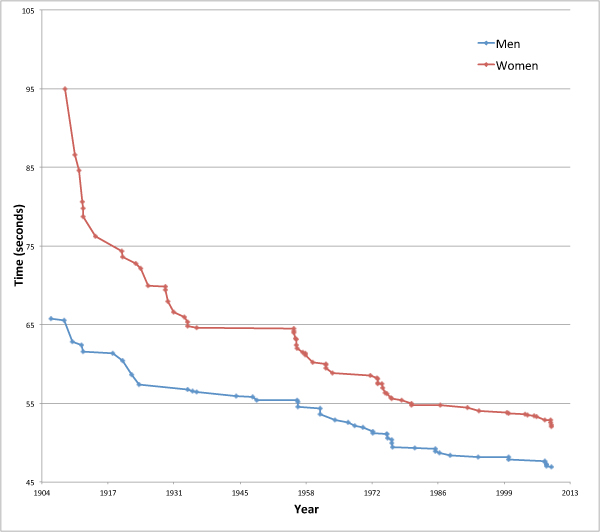
waves from adjacent lanes. (See below for a chart of world records over the 100 metre freestyle event since 1904.)

There are, broadly speaking, two things you can do to reduce your swimming time:
  1. Increase your power
  2. Reduce your drag
The magnitude $F_ D$ of the drag force acting on a swimmer moving in a fluid is given by the following equation

\[ F_ D=\frac{1}{2}\rho v^2 C_ D A, \]
where
  • $\rho $ is the mass density of the fluid
  • $v$ is the speed of the swimmer relative to the fluid
  • $A$ is the swimmer's cross-sectional area, that is the area of your body as it is pushing through the water head on
  • $C_ D$ is the drag-coefficient, a number which depends on factors such as the exact shape of the swimmer and the hydrodynamic qualities of their skin and what they are wearing.
Although it may seem like going to the gym and pumping some iron might be the obvious thing to do, reducing your drag is actually a speedier route to a quick lap time. Your power $P$ is the rate at which your body uses its energy, and when you are swimming the power you exert is proportional to the cube of your speed $v$

\[ P=F_ D v = \frac{1}{2}\rho C_ D A v^3. \]

Now suppose you want to increase your speed by 10%, from $v$ to $v+0.1v$. To do this solely by increasing your power, you need to exert a new power $P_1$
\[ P_1 = \frac{1}{2}\rho C_ D A (v+0.1v)^3. \]

The percentage increase in the power required is given by

\[ Increase = 100 \times \frac{P_1-P}{P}= 100 \times (\frac{P_1}{P}-1). \]

Since
\[ \frac{P_1}{P} = \frac{\frac{1}{2}\rho C_ D A (v+0.1v)^3}{\frac{1}{2}\rho C_ D A v^3}=(1.1)^3=1.331 \]

we have

\[  Increase =100 \times (1.331-1)\% =33.1\% . \]

So to increase your speed by 10% solely by increasing your power, you need to increase the power by 33.1%.

Reducing your drag is easier. From the equation for power above we see that the drag coefficient $C_ D$ is

\[ C_ D=\frac{2P}{\rho A v^3}. \]

Keeping your power output and cross-sectional area the same, increasing your speed by 10% requires a new drag coefficient $C_{D1}$ of

\[ C_{D1}=\frac{2P}{\rho A (v+0.1v)^3}. \]

The percentage decrease in drag coefficient is given by
\[ Decrease = 100 \times \frac{C_ D-C_{D1}}{C_ D}=100 \times (1-\frac{C_{D1}}{C_ D}) = 100 \times (1-\frac{1}{1.1^3})= 25\% . \]

So the 10% increase in speed requires a 25% reduction in the drag coefficient.

The exact same working can be used for cross-sectional area — a reduction of 25% will increase your speed by 10%. This is actually the key to the simplest method of reducing drag for most swimmers: improving your technique. Because human lungs are full of air, when we swim our upper body tends to rise and our lower body sinks, increasing cross-sectional area A. The drag force increases and you slow down. Keeping your feet nearer the surface is the easiest method of reducing drag for everyday swimmers.

Drugless doping


At the top end of competitive swimming nearly all swimmers already have very good techniques, so swimsuit technology comes into play. Materials have been developed that increase the swimmer's buoyancy, making it easier to keep their feet near the surface, and reduce the drag coefficient as the material glides through the water more easily than human skin does.

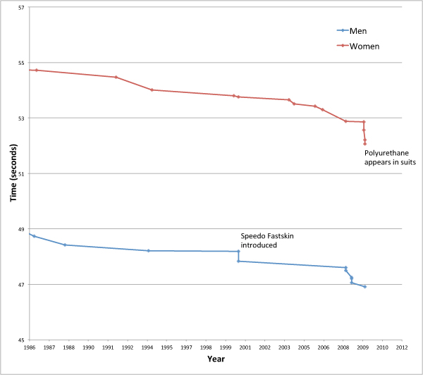
Full-length high-tech swimsuits were first introduced in 1999 before the 2000 Sydney Olympics, with the Speedo Fastskin suits containing V-shaped ridges, modelled on shark skin, to reduce drag. By 2008, the Speedo LZR Racer swimsuit was the most advanced. It was put through wind tunnel tests by NASA and mathematicians modelled water flow around it using a technique called computational fluid dynamics, which simulates how fluid flows around objects (see this article for more on modelling fluid flow). And this research all happened before real swimmers tested the suits in real pools. In Beijing, 89% of all swimming medals were won by swimmers wearing LZR Racer suits.
One of the ways the LZR Racer suits reduce drag is by having panels of a plastic called polyurethane on parts of the body that produce the highest drag. Other swimsuit manufacturers took note. Instead of being textile based with only patches of polyurethane, suits like the subsequent Arena X-Glide were made entirely of polyurethane. These suits were completely impermeable to water, so swimmers could conceivably complete their race without getting wet between their ankles and neck! Records continued to tumble. See more on the Speedo swimsuit technology in this article.

The governing body for swimming, FINA (Fédération Internationale de Natation – International Swimming Federation), took note of the plummeting records and the accusations of "technological doping". In March 2009 it put limits on the suits' thickness and buoyancy, affirming that "FINA wishes to recall the main and core principle that swimming is a sport essentially based on the physical performance of the athlete." They also stipulated that the suits should not cover the neck, shoulders and ankles.

This edict did not actually ban any of the new suits at the 2009 World Aquatics Championships (the "plastic games") — 38 meet records were broken. Subsequently all body-length swimsuits were banned. It was ruled that men's swimsuits may only cover the area from the waist to the knee, and women's from the shoulder to the knee. FINA also ruled that the fabric used must be a textile and not polyurethane. Despite these new rules, the records set by the now banned swimsuits were not revoked and still stand.

And as the term "textile" is not defined, and as scientists are pretty clever folk, the ambiguity of the new rules leaves open a large area for swimsuit development.

Record history


The progression of world records over the 100 metre freestyle event is shown below. Apart from some of the pool changes mentioned earlier, records have continued to drop as we increase our understanding of our physical abilities. Other innovations which have helped reduce times include the introduction of diving blocks in 1936 – previously swimmers had just dived from the wall – and the development of the tumble turn in the 1950s.

Records

It is interesting to note that freestyle as we know it now has not always existed. By definition, in freestyle races you can pretty much swim however you like (with some exceptions), unlike breaststroke, butterfly or backstroke which have defined methods of swimming. During the 1840s, even though they were beaten by native North Americans swimming with a front crawl style, British gentleman swimmers (in an oh so British fashion) swam only breaststroke, considering the front crawl too splashy, barbaric and un-European. In the late 1800s, the quickest (British) freestyle was the Trudgen style, named after John Arthur Trudgen, whose stroke was a combination of side stroke and front crawl. The Australian Dick Cavill modified this style to something similar to what is seen today with his Australian crawl and set a new world record for 100 yards in 1902.

The figure below shows a close-up of times from the early 1980s. You can see the decline around 1999 when the first fast-suits came in, then the sharp decline in 2008. It is difficult to predict when the next dots on the curves will occur.

Zoom on times from 1980s

At the time of writing, Australians are the favourites for both the men's and women's 100 metre freestyle events, with James Magnussen and Matt Targett having recorded the quickest men's 100 metre times in 2012, and Melanie Schlanger the quickest women's time. The UK's Francesca Halsall is 5th so far this year in the women's event, however Simon Burnett in 39th would be doing well to make it past the heats in the men's.

Sunday, 6 May 2012

Travelling Salesman - the Movie

Science in the movies is a topic we've looked at a few times here on the blog. But this one is for the pure mathematicians. Check out this preview to the upcoming flick "Travelling Salesman".


I love these kinds of films - overly melodramatic acting, a slight misrepresentation of the science behind the plot (which is OK by me as this is a movie), government conspiracies, and mysterious music. The name "Travelling Salesman" comes from the famous mathematical Travelling Salesman Problem in which a salesman needs to visit a numerous destinations and wishes to do it in the shortest time. Whilst this may seem to be a simple problem, it is one of the most studied problems in mathematics. The more destinations involved, the more difficult to solve and in general there is no algorithm that can find the best answer. Brute force methods (that is, computing every possible solution and then finding the best) are computationally difficult, and with too many destinations, impossible. Hence mathematicians often use heuristics which find good, although not necessarily optimal, solutions quickly.

The premise of the movie is that the famous P vs NP problem has been solved. I'm not a pure mathematician, so I'll do my best here... P problems are those whose solutions can be found quickly (in Polynomial time, hence the P). NP problems are those whose solutions can not be found quickly, but if somehow a solution is produced using some extra information, it is easy to check that this solution is the best one (in polynomial time). Solving these problems take Non-deterministic Polynomial time - hence NP. A good example to show this is a jigsaw puzzle - finding a solution may be very difficult (and it's probably most accurate to image a blind person doing the puzzle), but it only takes a quick glance to see if any solution is correct.

The question that mathematicians ask is whether P=NP - which means, are there algorithms out there that solve seemingly NP problems in polynomial time? We haven't found any yet and mathematicians tend to think that P does not equal NP, but there is currently no proof. Proving this one way or the other is one of the seven Millennium Prize Problems selected by the Clay Mathematics Institute and carries a US$ 1,000,000 prize for the first correct solution.

But why do we care? One of the reasons is that modern cryptography is based on the fact that P does not equal NP - this is the premise of the movie. Modern codes start with a pair of large prime numbers p1 and p2 and multiply them together to give  m=p1p2. The number m is released to the public, but p1 and p2 are kept secret. To crack the code you have to find p1 and p2, given the value of m. It turns out that finding the prime factors of large numbers (100+ digits) is exceptionally difficult, although checking an answer is very easy. It is thought to be an NP problem. But if indeed P does equal NP, this suggests that out there somewhere is an algorithm that could solve this problem in quick time, meaning that modern encryption codes are vulnerable.

They don't give too much away in the preview, but I suspect what happens is they prove P=NP, although the example of looking for something hidden in the desert seems like a P problem (you just check out under each grain of sand, which would be easy, although it's a nice illustration of the problem). We stretch the science here a bit - even if you prove P=NP, you still need to find the appropriate algorithm for the problem, which has never been done. But hey, it's a movie, and we don't pull Terminator up on its stretching of science!

There is a very good write up of the P vs NP problem over on Plus - check it out, it does a much more thorough job than I do!

Saturday, 5 May 2012

Ep 145: Teleportation


Is teleportation possible in the real world, or only in the world of science fiction?

In this very special episode, Dr Boob takes the reigns and leads us on a journey through teleportation, whether or not physics allows it and even if it does, can we technologically achieve it? What are the implications if we recreate someone in another spot - what about their soul? Does such a thing exist? And even if you can technologically achieve this, is it possible to reanimate a copy of someone? What do you do with their original version, if you have simply copied them? This could be considered cloning, which brings in ethical questions.

Perhaps wormholes could be a solution to this problem, but we haven't found any yet - however they are, as physicists like to say, theoretically possible.

Tune in to this very entertaining episode (and I can say this without any false modesty as Dr Boob did it all himself) here.


If you'd like to hear more of Dr Boob on this podcast, check out our past joint episodes, mostly on the science of superheroes. He's also on twitter, so come and follow him, he needs friends!


Thursday, 26 April 2012

Ep 144: Two-up - an ANZAC Tradition

2012 update: I had a chat to Chris Coleman of ABC Riverina about the maths behind two-up. Check it out here and read on for the 2009 article on the maths.

It's an Australian tradition on ANZAC Day to take yourself down to your local pub and play Two-up - an Aussie gambling game in which you toss two coins in the air and bet on the outcome.

I'm somewhat embarrassed to say that even though I am only a month away from turning 30, this year was the first time I've ever actually gambled on two-up.

It's not a game that is played very often, despite being iconically Australian - according to the GAMBLING (TWO-UP) ACT 1998, outside of casinos it is only legal to play two-up on commemorative days like ANZAC Day (unless you're in Broken Hill, where the local council can legally arrange a two-up game any day of the year).

The rules of two-up are pretty simple. The Spinner places two coins (traditionally pennies) on a small piece of wood (the kip) and tosses the coins into the air. In the version of two-up we played at the pub, the gambling was very simple. Players standing around the Spinner either gambled on HEADS - which is where both coins come up heads - or TAILS - which is where both coins come up tails. If a head and a tail come up, the coins are tossed again and no one wins or loses. To bet, you find someone else willing to gamble the same amount but opposite to you, and then you have a one-on-one contest. If you want to bet $10 on HEADS, then you find someone willing to bet $10 on TAILS, and if you win you get their $10 - if you lose, you hand over $10. It's very simple and I love its inbuilt honour system.

The probabilities involved are simple too - you have a 50% chance of winning each time you bet. At the start of our ANZAC day down in Balmain, most people were betting $5. By the end of the day, as more beers were consumed, many were betting $50 and $100. Gambler's Ruin also started to show it's head - many people think that by doubling your bet after you lose you can get yourself back into the game. This doesn't work in this form of two-up for a couple of reasons. The first is that you need to find someone willing to bet the same amount as you, which is increasingly unlikely the larger you want to bet. And secondly, unless you have unlimited funds (or strictly speaking, more than everyone else you could bet against - or the casino if you are gambling there), it is highly unlikely that you could continually bet without going out backwards.

Two-up is also played in casinos and other gambling houses, and not just on ANZAC day. The rules, as you would expect from such institutions, are not so simple. In this expanded form of the game, there are a number of ways to bet. The South Australian Government has a good guide to two-up play, but simply put:

Players can bet in the following ways:

1) HEADS - odds of 1/1 ($1 bet pays $2, including your original $1);
2) TAILS - odds of 1/1;
3) 5 consecutive ODDS - odds of 25/1 ($1 bet pays $26).

The Spinner can bet in the following ways:

1) 3 HEADS are thrown before TAILS is thrown and before 5 consecutive ODDS are thrown - odds of 7.5/1 ($1 bet pays $8.50);
2) 3 TAILS are thrown before HEADS is thrown and before 5 consecutive ODDS are thrown - odds of 7.5/1.

This makes the game a little bit more interesting. The Wizard of Odds website for two-up sets out the probabilities for each of these outcomes - let's derive where they come from. At each toss of the kip, for this analysis it is best to think of there being 3 possible outcomes - HEADS, TAILS or 5 consecutive ODDS. We think of it this way because if a single ODDS is thrown, it is re-thrown and only makes a difference if it is one of five in a row.

Player Odds:

As you can see, the House is paying out as if the odds are better than they actually are. It's not much, but this is how they make their money.

Spinner Odds:

Again we can see, the House is not paying enough for a win - the odds should be 7.8 to 1, rather than 7.5 to 1. However, were you to back HEADS on each throw rather than as the group of three, the house would offer you odds of 7 to 1 (this is left as an exercise for the reader...), so the spinner's bet is better.

As it turns out, I came out even at the end of the day! There's some more maths to be had here - sometime soon we might take a look at some of these pay-out distributions.