My favourite Sesame Street science videos

I'm stranded at Adelaide airport with my flight delayed for four hours, so what better way to get back onto the blog than by sharing my favourite Sesame Street science videos (Sesame Street having recently resumed it's exalted position in my life). The other day they were using the scientific method to deconstruct fairy tales - how would you tell the difference between the Big Bad Wolf and Grandma? Those videos aren't up online yet, but let's kick this off with comedian Craig Ferguson helping to define the word "experiment".



Here's Elmo and a Justin Bieber look-alike singing "Measure, Yeah, Measure," to the tune of Bieber's song "Never Say Never." I like his hair flicks. Elmo measured it, yo.



This is pretty cool, a Cookie Monster interactive video teaching us about experiments and things that float:



In this one, Emma Stone balances stuff on her head:



Here's Ernie showing all the curiosity of a good scientist:



And this is not sciencey, but it's the best Sesame Street video. Cutest thing you will ever see!

The 27 Club

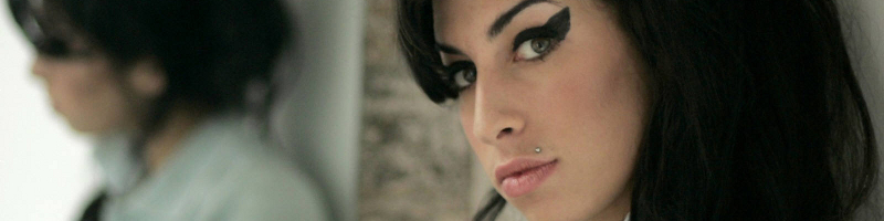
Brian Jones, Jimi Hendrix, Janis Joplin, Jim Morrison, Kurt Cobain, and this week tragically Amy Winehouse, all died at the age of 27. This coincidence has spawned the notion of the 27 Club - a club whose members are influential musicians who died at the age of 27. But is there anything statistically significant about this club? Should musicians fear turning 27?

There are a few things that we should note before starting this investigation:

1. It's quite clear that it is not true to say that more influential musicians die at the age of 27 than at any other age. If this were true, musicians would be dying all the time, and the facts that our radios are filled with golden oldies and John Farnham keeps touring are testament to this. 
2. We will never find enough data to fully test out any theory we come up with. For example, what defines an "influential" musician? One approach might be to scour wikipedia and find the death dates of every artist who had a top ten hit in the last 50 years. I leave this as an exercise for the reader.

What we will do for this article is redefine the club to be for musicians who have died through misadventures with drugs. And what do you know, wikipedia has an article dedicated to just this topic - a list of celebrities who had drug-related deaths. Looking at just the 100 musicians in the list, we get the following distribution for lifespans of musicians who died through drug misadventure.

This distribution has an average of 36, a median of 34 and a mode of 28. All pretty close to 27. Maybe there's more to this than we thought. This can be compared to Australian Bureau of Statistics data for Australian males between 2007 and 2009. It's clear that musicians who have drug-related deaths are dying at a much younger age than Australian males. Note the caveat here, the musicians aren't dying of old age - these are only musicians who have drug-related deaths.


It's easy enough to come up with a theory for this. Musicians - indeed society at large - are most likely to start being exposed to drugs at the age of 20. In any case, before this time there aren't many musicians popular enough to have a wikipedia page or a public influence strong enough to be accepted into the 27-Club. The number of deaths seems to drop off after about the age of 40, but this is not because they are all becoming family oriented and leading a clean life. The number drops because there are less musicians alive at 40 to die. This is the same explanation for why less people in the general population die at the age of 95 than do at 80 - not that many people live long enough to die at 95.

The following chart displays the probability of dying within the next five years given that you have survived to now. For example, if you are currently in the 60-64 year age range, this chart shows the probability of dying in the 65-69 year age range. For musicians who have drug-related deaths, between the ages of 20 and 65, the chance of dying in the next 5 years is between 25-50%. Within the noise of the small sample set, its about the same for each 5 year category between 20 and 65, perhaps increasing slightly with age. This suggests that for influential musicians, if they are going to die through drug use, they have roughly the same chance of dying within the next 5 years no matter how old they currently are, perhaps a little higher if they're older. The probability of death doesn't peak at 27, and conversely, just because you have survived till now doesn't mean you have a greater chance of surviving the next five years. This is similar to the distribution of cricket batting scores, for those interested.

The peak at 25-29 in the previous chart occurs only because the musicians have not died before that age and suggests there is nothing supernatural about the number 27 (despite the curse of 27). Note that for Australian males, the data stops at 100 so the 100+ bar represents dying above this age. For the musicians, the data stops at 70-74, hence its peak at 100%.




Note again that this analysis is for musicians who die drug related deaths. It doesn't suggest that musicians have shorter lifespans than the average Australian male - it does however suggest that musicians who die via drugs have shorter lifespans. This could be because if you are going to die a drug-related death you are likely to die young because taking drugs is a risky endeavour, or it could be because by the age of 75 you have probably stopped doing drugs and so your death doesn't appear in the chart.

So is there anything to the 27 club? Not really. We've shown (albeit with just one rather incomplete article on wikipedia) there is nothing magical about the age of 27 - indeed 28 seems more interesting - and the peak in drug-related deaths around this age is quite predictable. Far more musicians die at an older age of other causes just like the rest of us, and somehow Keith Richards is still alive. The club exists because humans like to associate meaning to patterns. We're very good at pattern recognition. Our ability to associate the seasons with animal migrations, and the stars in the sky with when to plant vegetables, gave us an advantage throughout evolution. However, false pattern recognition doesn't get us killed and so we often spot patterns where they don't exist - for example, we see faces in the World Trade Center disaster, or the Virgin Mary at the beach. Some even believe that because of this, we have created religion to explain patterns we can't explain.

A nod here to the like-minded Bespoke Blog and its article Morbid Statistics & The 27 Club which I found quite coincidentally as I was finishing up this article. 

Ep 143: TedxSydney - Bryan Gaensler

TED is a US based not-for-profit enterprise devoted to the propagation of Ideas Worth Spreading. TED started out in 1984 as a conference bringing together people from three worlds: Technology, Entertainment and Design. TedxSydney was a Sydney-based TED event, bringing people together to share a TED-like experience. I ducked out to Carriage Works to catch some of the event, and you can see all the talks over at the TedxSydney youtube channel. Many of these talks were science based, so I'm going to put up some of my favourites over the next few posts.

The following video is from Bryan Gaensler, former Young Australian of the Year, NASA Hubble Fellow and Harvard professor, Australian Laureate Fellow at The University of Sydney, and Director of the Centre of Excellence for All-sky Astrophysics. His talk was entitled A new way of looking at the sky.

Ted Copyright
TEDTalks are distributed under a Creative Commons (CC) license. Anyone is free to download the videos from TED.com; share them with friends; republish or embed them on their website or blog. But this use must be made within the terms of the CC license "Attribution -- NonCommercial -- NonDerivative."

Ep 142: Beyond Zero Emissions

Beyond Zero Emissions is a not-for-profit, volunteer run organisation whose core goal is to develop blueprints for the implementation of climate change solutions. In partnership with the University of Melbourne's Energy Research Institute, BZE are undertaking the Zero Carbon Australia 2020 Project, which puts together fully costed transition plans for getting Australia to zero emissions in ten years using commercially available technology.

Last year I attended their launch event for the Zero Carbon Australia Stationary Energy Plan which goes into detail about how Australia can reach 100% renewable energy within a decade. Speakers at the launch included former NSW premier Bob Carr, member for Wentworth Malcolm Turnbull, Greens Senator Scott Ludlam and Matthew Wright, Executive Director of BZE. The event was hosted by journalist Quentin Dempster.

In this podcast, with permission from Matthew Wright, I bring you Matthew's speech at this launch which details the science behind their proposal. I also chatted to BZE volunteer Petra Liverani at the recent Say yes to a price on carbon pollution rally in Sydney.

Click play below or listen to this show here:



If you'd like to hear what Turnbull, Carr and Ludlam had to say, check out the full video of the launch below, reproduced here with permission.

Total lunar eclipse across Australia (or what is a syzygy)

Today I learnt a new word.

Syzygy.

A syzygy is a straight line configuration of three celestial bodies (such as the Earth, Sun, and Moon), and on Thursday 16 June, if you can get yourself up before dawn, you will witness a syzygy - in this case a total lunar eclipse - above the western horizon as the Moon passes through Earth’s shadow. This syzygy ends at sunrise in all states but Western Australia. It has been something of a star and planet watcher's dream recently, with four planets having lined up in the sky during May.

The eclipse begins at 3:25am AEST and enters its darkest phase at 05:22am AEST when the transformation to a blood-red Moon should begin. The colour of the eclipse depends on the amount of dust in the Earth's atmosphere. The red colour comes about because sunlight reaching the Moon passes through the Earth’s atmosphere where it is scattered. Shorter wavelengths (blue) are scattered more by  air molecules and dust particles than longer wavelengths (red), and so by the time the light has passed through the atmosphere, the light is mainly red. In extra-solar planets - planets in other solar systems - lunar eclipses can be used to determine the content of the planetary atmosphere. You might remember back to 2009 when Sydney was covered in dust and turned red to gauge a feeling for what the colour could be like - check out that article for a fuller description of the physics involved as it is similar.

If you are keen enough to not only get out of bed but to leave your house, Sydney Observatory is hosting a special breakfast viewing which includes tea, coffee, croissants and “blood-red” jam. Book at the Sydney Observatory website.

This material came from the Sydney Observatory.

There is more kicking in Union than League (and other misconceptions)

If you listened to the crowd at a Waratahs (Rugby Union) game, apart from wondering which side the so-called fans were barracking for, you'd think that the Waratahs kicked the ball too much. If you have ever listened to a Rugby League fan wax lyrical about how Union teams keep kicking the ball away and how League teams know how to cross the try line, you might start to become convinced that Union teams really do kick too much. But as we like to do here, let's put these popular notions to the test. Is there really more kicking in Union than League?

The question originated at my work, where most Mondays - indeed most days of the week - we debate the relative merits of the two rugby codes. So if for no other reason than to prove my own hunch, I compiled the data for the current season of the Australian National Rugby League (after round 12) and the three nation Super Rugby (after round 15) tournaments. The following chart shows the distribution of the number of times each game a team kicks the ball.


We can conclude:

• This year in the NRL, each team averages 19.05 kicks per game. In Super Rugby, each team averages 19.07 kicks per game - there is essentially no difference between the average number of kicks in a Union game and a League game in 2011. The difference of 0.02 is well below what we need for statistical significance;
• Both sets of data look pretty-much bell shaped - that is, they are close to normal distributions (probably as a result of the Central Limit Theorem). The League distribution is thin and tall - there is only a small distribution about the mean (standard deviation of 3.8) - whilst the Union distribution is fatter (standard deviation of 6.2). This suggests that in a League game, most of the time teams will kick somewhere near this average number of times (19), whilst in a Union game you are more likely to see a game with not many kicks or a game with a lot of kicks. This is a result of the fact that in League, after the 5th tackle, you don't have many other options but to kick, whilst in Union, with an unlimited tackle count and continual contest for the ball, you have more options for when and how often you wish to kick.
• The notion that it's the boring teams that kick too much take another hit when you look at the teams who actually do kick the most. The Reds, lauded this year for playing running rugby, are top of the kick table, whilst the Brumbies, who can't beat anyone, are stuck at the bottom of the kick and Super Rugby tables. In the NRL, the top three kicking teams are 3 of the top teams in the competition. Check out Green and Gold Rugby for more on the Super Rugby kicking stats.
  
  

  Super 15			NRL
  Reds	23.8		Dragons	21.9
  Waratahs	22.8		Storm	20.6
  Cheetahs	21.1		Broncos	20.5
  Rebels	20.7		Eels	20.4
  Stormers	20.1		Sea Eagles	20.2
  Bulls	19.9		Warriors	19.4
  Sharks	18.9		Raiders	19.4
  Force	18.7		Rabbitohs	19.4
  Blues	18.6		Sharks	19.2
  Chiefs	18.6		Knights	19.2
  Crusaders	17.4		Cowboys	18.6
  Hurricanes	17.2		Panthers	18.2
  Lions	16.5		Bulldogs	18.2
  Highlanders	16.4		Titans	17.7
  Brumbies	14.5		Roosters	16.5
  			Wests Tigers	15.6

 
• I find it fascinating that the averages come out so close. It's over 100 years since the codes split from their common ancestor, and despite numerous law changes and evolutionary paths, teams in League and Union seem to want to hold onto the ball, on average, for about the same amount of time. In league, you are limited to 6 tackles, so could it be that the law-makers of League, when devising the 6 tackle rule, knew instinctively that this is the right balance of attack and defence? Does this balance give the players just the right amount of rest during a game? Or is it all a coincidence?

And while we're on the topic of maths and sport, it's important when doing statistical analysis on sport that you analyse the right thing and take note of statistical significance. Despite the popular saying, statistics don't lie, but poor use and interpretation of them does. I think this comic from xkcd sums up how I feel when I listen to ex-professional sportsmen commentating on sport...



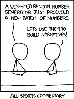
With regards to cricket, we have shown here on the blog that a batsman's cricketing scores over his career fit the exponential distribution very well, suggesting that many notions of cricketing form, and discussions of it, are quite troublesome - that is, it's not form creating the fluctuations in a batsman's career, but the very nature of the game itself. Deep.

Kicking images courtesy State of Union address - Tom Bradshaw's rugby blog. Yes I support the Waratahs and believe wholeheartedly that Rugby Union is a much better game than League. And unlike other Waratahs fans, I think they're actually pretty good!

How the planet alignment worked (and why astrology does not)

Did you get up at 5am and brave the cold to see the planets align? If you had, you would have seen something like this. Venus and Jupiter were very bright, Mercury was fainter and eventually fell behind some clouds, and I couldn't see Mars at all with the naked eye. It was only with this long exposure shot that I could see what I think to be Mars. I've put up a bunch of photos on flickr.



The reason we were treated to this early morning light show was because of a rare alignment of the planets. It's not rare due to being unexpected - it's completely predictable - it just doesn't happen all that often. The next time these four planets will get together will be in 2056.

The following images have been made using the excellent Solar System Live by John Walker. The site shows the positions of the planets around the Sun, and in the sky, either live or at a time of your choosing. On May 13, the four inner planets were all in a straight line and from Earth you could view the other three clumped together in the sky. The images show the solar system from above, with the orbits spaced equally for ease of viewing. From this viewpoint, the Earth spins counter-clockwise on its axis, and counter-clockwise around the Sun. The alignment of planets is not seen until just before dawn, however as the Earth continues to rotate and the Sun comes into view, the light from the Sun becomes too strong to see the planets (you rarely see stars or planets during the day). Unseen, they continue to track overhead during the day. By the end of May, as the various planets move at different orbital speeds around the Sun (a year is different on each planet), they will be in different parts of the sky and the light show over.



If you take a closer look at the figure below, you'll notice that besides the aligned planets, there are actually six planets visible in the dawn sky - all planets except Saturn can be spotted if you find a dark enough area, although you'll need binoculars to see Uranus and Neptune. Even Pluto, if you still maintain it to be a planet, might be found with a small telescope - the Solar System live site still has Pluto in its diagrams. A crescent Moon will reappear near the end of May to add to the scenery.



For more information, this video from ScienceCasts gives a great overview of the phenomenon, showing how the planets move in the sky throughout May. It's also a geometry lesson before breakfast. Check out science.nasa.gov for more.



Astrology
The alignment of the planets has various meanings in astrology and some astrologists maintain that there is science behind their beliefs, often claiming the precise positioning of the planets and stars at your birth effects you through gravity. Whilst these effects may be small, some claim they're enough to influence your developing brain and therefore your personality. Let's test the theory. To find out the gravitational force between two masses, we use Newton's law of universal gravitation:



where:

• F is the force between the masses,
• G is the gravitational constant,
• m₁ is the first mass,
• m₂ is the second mass, and
• r is the distance between the masses.

We can use this to examine the gravitational force between a one kilogram mass on the surface of the Earth and the distant planets. The distances the planets were from Earth on May 13 were obtained from Solar System Live, and their masses from NASA. I've also included the gravitational effect of my car if you were standing 50 cm from it.

As you can see, the gravitational effect of my 1.5 tonne car is greater than all the planets put together.

It is also important to note that on May 13, the pull of the Moon on our 1kg object was 199 times bigger than that of Jupiter's at the Earth's surface. The Sun's pull was 178 times bigger than the Moon's, and the pull of the Earth itself was 1656 times bigger than the Sun's. Essentially, the pull of the planets on an object at the Earth's surface is negligible. The calculations can be explored in this spreadsheet. Read more over at Bad Astronomy debunking the claims of astronomy, especially with regards to gravity and the tides.

So, don't blame Jupiter if luck doesn't favour you this month - blame my car. Oh Marc, that is such a Taurian thing to say...

Four planets align over Sydney at dawn Friday 13 May

When the moon is in the Seventh House
And Jupiter aligns with Mars
Then peace will guide the planets
And love will steer the stars.

The age of Aquarius has arrived! Well, it will, this Friday 13th May.

In a rare planetary event, Mercury, Venus, Mars and Jupiter, will appear together (within around 2 degrees of each other) in the eastern sky just before dawn this Friday. The event will be particularly spectacular for Sydneysiders. From 5am, the four planets will be clearly seen just above the horizon in the east. The brightest planet will be Venus sitting in the middle of the group. Just above and to the left of Venus and almost as bright is Jupiter. To the right of Jupiter and slightly fainter will be Mercury. Sitting below these three planets and fainter again will be Mars. The four planets are quite bright, so if you are up early enough, you will see them over city lights.

If you have been up early recently (I had the pleasure of a 5am start today for work...) you will have already noticed Venus and Jupiter together. The last time these four planets came together was in 1910, but the planets were too close to the Sun to observe. The next close grouping of these planets will not be until 2056.

“The close grouping of these particular four planets only happens every 50 to 100 years. We are hoping for a clear autumn morning for this unique sight in the southern sky,” said Sydney Observatory’s acting curator, Andrew Jacob. The event will be visible to the naked eye and Sydney Observatory is holding a breakfast viewing. If you are interested in getting along, there is more information at www.sydneyobservatory.com.au, and check out the Observatory's blog.

The last cool astrological event that we've seen in Sydney was back in 2008 when the Moon, Venus and Jupiter aligned to form a smiley face in the sky. I was a bit late for the happy face but managed to capture a grainy celestial sad face. Time will tell whether I manage to drag myself out of bed at 5am for this latest viewing - with a new born bub, you never know...

Addendum: Here's an explanation of how the alignment gave such a great view from Earth, and why my car is more likely to influence your personality - astrologically speaking - than this rare alignment.

Ep 141: Science of Superheroes - Harry Potter

And we're back! It's been a while, but finally it's time for another podcast, so we've made it a long one. Take this episode on a long train ride or car trip, as Dr Boob and I explore the science of the spells of Harry Potter.

Attempting to find scientific and engineering solutions to Harry Potter spells is probably the most difficult task we have set ourselves yet, so we would be very interested to hear how you would made the Harry Potter spells a reality. The spells dealt with in this episode are:

1. Lumos - Producing light from the end of a wand (A voice activated torch seems a logical solution),
2. Aguamenti - Shooting water from the end of the wand,
3. Alohomora - Picking a lock at a distance,
4. Expecto Patronum - Protection against evil dementors in the form of some virtual creature,
5. Sectumsempra - Slicing your opponent open,
6. Aparecium - Reading invisible ink,
7. Accio - Summoning things to you,
8. Expelliarmus - Disarming your opposition of their wand,
9. Confundo - Confusing the victim,
10. Stupefy - Stunning the victim,
11. Invisibility cloak - Covering yourself in a cloak to make yourself invisible,
12. Imperio - Forcing your victims to obey your commands,
13. Obliviate - Erasing the memories of the victim,
14. Legilimens - Telepathy.

Although some of these are quite clearly impossible at the moment, in every case we have come up with a scientific or engineering solution to take us at least part of the way there. Listen in to find out what we came up with, and please write in and let us know where we have gone wrong or what you would do.

Click play below or listen to this show here.



References:

1. Santos, V., Paula, W., & Kalapothakis, E. (2009). Influence of the luminol chemiluminescence reaction on the confirmatory tests for the detection and characterization of bloodstains in forensic analysis Forensic Science International: Genetics Supplement Series, 2 (1), 196-197 DOI: 10.1016/j.fsigss.2009.09.008
2. A.J. Barnier and D.A. Oakley (2009). Hypnosis and Suggestion Encyclopedia of Consciousness DOI: 10.1016/B978-012373873-8.00038-4
3. T.C. Jerram (1982). Hypnotics and sedatives Side Effects of Drugs Annual DOI: 10.1016/S0378-6080(82)80009-3
4. Wood, B. (2009). Metamaterials and invisibility Comptes Rendus Physique, 10 (5), 379-390 DOI: 10.1016/j.crhy.2009.01.002

Are NSW players over-represented in the Australian cricket team?

In every sports competition in the world, fans of one team will claim another team gets more favourable treatment than their own, whether it’s selection in representative teams, concessions regarding player salaries or favourable refereeing decisions. Cricket in Australia is no different. The dawn of summer is almost inevitably accompanied by bleating, generally from Victorian fans, about how players from New South Wales are more likely to be selected in the national team than players from other states. This opinion found a voice in David Hookes, who claimed:

"When they give out the baggy blue cap in New South Wales, they give you a baggy green one in a brown paper bag as well to save making two presentations."

It’s about time we put this idea to the test. Since the 1977/78 season, all 6 Australian states have played in the Sheffield Shield, Australia’s domestic first-class cricket competition. Since 1982/83, the season has culminated in a grand final (previous to this the winner was determined league style by whoever won the most throughout the season). I will use data from 1982/83 till now for consistency and so that all states are represented. The following table shows the players who have debuted for Australia since the start of the 1982/83 season, the state they were playing for at the time of their debut, and the number of Tests they played throughout their career.

Player	Years	Tests	State		Player	Years	Tests	State
Carl Rackemann	1982–91	12	Qld		Matthew Elliott	1996–2004	21	Vic
Kepler Wessels	1982–85	24	Qld		Michael Kasprowicz	1996–2006	38	Qld
Tom Hogan	1983–84	7	WA		Jason Gillespie	1996–2006	71	SA
Roger Woolley	1983–84	2	Tas		Andy Bichel	1997–2003	19	Qld
Wayne B. Phillips	1983–86	27	SA		Shaun Young	1997	1	Tas
John Maguire	1983–84	3	Qld		Simon Cook	1997	2	NSW
Greg Matthews	1983–93	33	NSW		Stuart MacGill	1998–2008	44	NSW
Steve Smith	1984	3	NSW		Gavin Robertson	1998	4	NSW
Dean Jones	1984–92	52	Vic		Paul Wilson	1998	1	SA
David Boon	1984–96	107	Tas		Adam Dale	1998–99	2	Qld
Bob Holland	1984–86	11	NSW		Darren Lehmann	1998–2004	27	SA
Murray Bennett	1984–85	3	NSW		Colin Miller	1998–2001	18	Tas
Craig McDermott	1984–96	71	Qld		Matthew Nicholson	1998	1	WA
Simon O'Donnell	1985	6	Vic		Adam Gilchrist	1999–2008	96	WA
Dave Gilbert	1985–86	9	NSW		Scott Muller	1999	2	Qld
Robbie Kerr	1985	2	Qld		Brett Lee	1999–2010	76	NSW
Merv Hughes	1985–94	53	Vic		Simon Katich	2001–	56	WA
Geoff Marsh	1985–92	50	WA		Martin Love	2002–03	5	Qld
Bruce Reid	1985–92	27	WA		Brad Williams	2003–04	4	WA
Steve Waugh	1985–2004	168	NSW		Nathan Bracken	2003–05	5	NSW
Simon Davis	1986	1	Vic		Andrew Symonds	2004–09	26	Qld
Tim Zoehrer	1986–87	10	WA		Michael Clarke	2004–	67	NSW
Chris Matthews	1986–88	3	WA		Nathan Hauritz	2004–	17	Qld
Greg Dyer	1986–88	6	NSW		Shane Watson	2005–	25	Qld
Peter Taylor	1987–91	13	NSW		Shaun Tait	2005–08	3	SA
Mike Veletta	1987–90	8	WA		Michael Hussey	2005–	57	WA
Tim May	1987–95	24	SA		Brad Hodge	2005-08	6	Vic
Tony Dodemaide	1987–92	10	Vic		Phil Jaques	2005–08	11	NSW
Ian Healy	1988–99	119	Qld		Stuart Clark	2006–09	24	NSW
Trevor Hohns	1989	7	Qld		Dan Cullen	2006	1	SA
Mark Taylor	1989–99	104	NSW		Mitchell Johnson	2007–	40	Qld
Greg Campbell	1989–90	4	Tas		Chris Rogers	2008	1	WA
Tom Moody	1989–92	8	WA		Brad Haddin	2008–	30	NSW
Mark Waugh	1991–2002	128	NSW		Beau Casson	2008	1	NSW
Shane Warne	1992–2007	145	Vic		Cameron White	2008–09	4	Vic
Wayne N. Phillips	1992	1	Vic		Peter Siddle	2008–	20	Vic
Paul Reiffel	1992–98	35	Vic		Jason Krejza	2008	2	Tas
Damien Martyn	1992–2006	67	WA		Doug Bollinger	2009–	12	NSW
Justin Langer	1993–2007	105	WA		Andrew McDonald	2009	4	Vic
Jo Angel	1993–95	4	WA		Ben Hilfenhaus	2009–	15	Tas
Michael Slater	1993–2001	74	NSW		Phillip Hughes	2009–	8	NSW
Brendon Julian	1993–95	7	WA		Marcus North	2009–	21	WA
Glenn McGrath	1993–2007	124	NSW		Bryce McGain	2009	1	Vic
Matthew Hayden	1994–2009	103	Qld		Graham Manou	2009	1	SA
Michael Bevan	1994–98	18	NSW		Clint McKay	2009	1	Vic
Damien Fleming	1994–2001	20	Vic		Ryan Harris	2010–	4	SA
Phil Emery	1994	1	NSW		Tim Paine	2010	4	Tas
Greg Blewett	1995–2000	46	SA		Steven Smith	2010–	3	NSW
Peter McIntyre	1995–96	2	SA		Peter George	2010–	1	SA
Stuart Law	1995	1	Qld		Xavier Doherty	2010	2	Tas
Ricky Ponting	1995–	151	Tas		Michael Beer	2011–	1	WA
Brad Hogg	1996–2008	7	WA		Usman Khawaja	2011–	1	NSW

Of the 104 players who debuted after 1982/83, 28 were playing for NSW when they were first picked for Australia (27% of the new players).

	Players	Percentage
NSW	28	27%
WA	20	19%
Qld	18	17%
Vic	16	15%
Tas	10	10%
SA	12	12%

Clearly NSW players have played more Tests. But is this unreasonable? There are two measures we can look at here. Sheffield Shield results and state populations. The following shows the results of the Shield since 1982/83.

Season	Winner	Second	Third	Fourth	Fifth	Sixth		Season	Winner	Second	Third	Fourth	Fifth	Sixth
1982–83	NSW	WA	SA	Tas	Qld	Vic		1997–98	WA	Tas	Qld	NSW	Vic	SA
1983–84	WA	Qld	Tas	NSW	SA	Vic		1998–99	WA	Qld	Vic	SA	Tas	NSW
1984–85	NSW	Qld	SA	WA	Vic	Tas		1999-00	Qld	Vic	WA	SA	Tas	NSW
1985–86	NSW	Qld	Vic	WA	SA	Tas		2000–01	Qld	Vic	NSW	Tas	WA	SA
1986–87	WA	Vic	Qld	SA	NSW	Tas		2001–02	Qld	Tas	WA	SA	Vic	NSW
1987–88	WA	Qld	NSW	Vic	SA	Tas		2002–03	NSW	Qld	Vic	SA	WA	Tas
1988–89	WA	SA	Qld	NSW	Tas	Vic		2003–04	Vic	Qld	Tas	WA	NSW	SA
1989–90	NSW	Qld	SA	Tas	WA	Vic		2004–05	NSW	Qld	WA	Vic	SA	Tas
1990–91	Vic	NSW	Qld	WA	SA	Tas		2005–06	Qld	Vic	SA	Tas	WA	NSW
1991–92	WA	NSW	Vic	Qld	SA	Tas		2006–07	Tas	NSW	Vic	Qld	WA	SA
1992–93	NSW	Qld	WA	SA	Tas	Vic		2007–08	NSW	Vic	WA	Tas	SA	Qld
1993–94	NSW	Tas	WA	Vic	SA	Qld		2008–09	Vic	Qld	SA	Tas	WA	NSW
1994–95	Qld	SA	Vic	WA	NSW	Tas		2009–10	Vic	Qld	NSW	WA	Tas	SA
1995–96	SA	WA	Qld	Tas	NSW	Vic		2001–11	Tas	NSW	Qld	WA	Vic	SA
1996–97	Qld	WA	NSW	Tas	Vic	SA

NSW has won 9 Shields, ahead of WA’s 7. If you look at the percentage of Shield wins per state and compare this to the number of players picked for Australia from that state, you will notice that these results are remarkably similar. Is it any surprise that the most successful team over this time has more players picked for representative honours? If you look at all the Tests played since 82/83, 34% of the Test positions up for grabs were occupied by NSW players, and the order of states is exactly the same as the order for number of Shield wins. This is strong evidence that rather than a selection bias, players are being picked either because they are the best players or because they have been a part of successful teams.

	Players			Tests			Shield wins
NSW	28	27%		983	34%		9	31%
WA	20	19%		540	18%		7	24%
Qld	18	17%		516	18%		6	21%
Vic	16	15%		380	13%		4	14%
Tas	10	10%		306	10%		2	7%
SA	12	12%		208	7%		1	3%

The second way to look at this is by state population. I don’t particularly like this method because sportsmen, especially in this professional age, move teams for many reasons, including for better opportunities and more pay, and don’t necessarily play for the state of their birth. The most populous state is not necessarily going to have the best team. But because this is often the first measure people look to when analysing team results (for example, Olympic results), and because arguably a larger population means a bigger economy and therefore more money flowing through the team, we shall include some analysis. Since 1982, NSW (+ACT) has averaged 36% of the total population of the states (excluding Northern Territory). Again, this matches quite closely the number of players picked for Australia – indeed, you might argue that more players from NSW should have been picked. It would be by this measure that Victorians may claim some bias.

	Population	Shield Wins
NSW + ACT	36%	31%
Vic	25%	14%
Qld	18%	21%
WA	10%	24%
Tas	3%	7%
SA	8%	3%

Finally, let’s look at the one-test wonders – the players who only played one test.

	One Test wonders
NSW	3
WA	3
Qld	1
Vic	4
Tas	1
SA	4

Victoria and SA share this honour with 4 one-test wonders – and this is possibly why David Hookes, of SA stock and coach of Victoria after his retirement, was cranky. In the case of SA, this is a third of their players who have made their debut since 1982/83 – indeed, 7 of their 12 Test players did not play more than 4 Tests. Tasmanian players also fair poorly in this regard, with 6 of their 10 players playing no more than 4 Tests – Tasmanian results are severely skewed by Ponting’s 151 and Boon’s 107 Tests.

No matter what state a Test player is from, he has roughly the same chance of playing 15 or more Tests. Thus the data does not support the idea that selectors are more likely to stick with NSW players through a patch of poor form.

	Percentage of state Test players (15+ Tests)
NSW	43%
WA	40%
Qld	56%
Vic	44%
Tas	40%
SA	42%

I would be interested to hear your thoughts regarding this – I know it can stir some passions. But the data would suggest that there is no unfair bias towards NSW.

Further thoughts:

• I have made no attempt to look at players moving state during their careers. Simon Katich, for instance, had a career revival when playing for NSW, even though he was originally picked for Australia when playing for WA. Nathan Hauritz similarly had his fortunes revived when playing for NSW, even though he debuted when playing for Queensland. There are also many examples of this working the other way – Jason Krejza moved to Tasmania, and Adam Gilchrist to WA, both from NSW and then made their debut. Even Don Bradman first played for NSW before an ongoing career with SA.
• You could do the same analysis if you have time and patience on your hands for one-day and Twenty20 cricket.
• It was quite difficult in some cases to track which state a player was playing for when they made their Australian debut, especially if they moved state soon after. I have put the data here (some of the array formulae don't work in Google docs, and I have stripped out the macros, but you can redo them). If I have made a mistake, let me know!

Search Traffic in Egypt

The Egyptian Revolution of 2011 was a series of street demonstrations that demanded the overthrow of the Egyptian President Hosni Mubarak. One of the government retaliations to the protests was to shut down the Internet. Imagine you're a youth in Egypt and all of a sudden you don't have access to the Internet with its social networks, games and unlimited porn. You'd protest too! Great strategy guys...

Here is the Google search traffic in Egypt normalised against world-wide Internet traffic, created through Google Transparency Report. As you can see, it took a little less than a week for the government to realise their folly.

Science events for February, and a little bit of Valentine love

February is a big month for science, and a big month for love. Here are a couple of events that caught my eye.

Worldwide:

The Global Google Science Fair is an online science competition open to all students aged 13 to 18 from around the world. Unfortunately, I'm now way too old to enter, but were I still at school, this would be a fantastic opportunity to have some fun with science and technology. Scientific American, Lego, National Geographic and CERN are partners in the science fair, whose winner will receive a $50,000 scholarship, a 10-day trip to the Galápagos Islands and a virtual internship at Lego or a three-day site visit to CERN, Google or Scientific American.

The idea behind the show is that it is a chance for participants to showcase their ideas and experiments. Entrants are required to submit their work either as a video or slide show on their website (using Google products of course), and the works can fall into the following categories:

1. Computer Science & Math
2. Earth & Environmental Sciences
3. Behavioral & Social Sciences
4. Flora & Fauna
5. Energy & Space
6. Inventions & Innovation
7. Physics
8. Biology
9. Chemistry
10. Food Science
11. Electricity & Electronics

Check out the Official Rules carefully and watch the video below for an introduction:



Sydney:

The Powerhouse Museum is opening three new exhibitions in February and March 2011. The exhibitions, Engineering Excellence (open now), designTECH (opens 19 February) and Student Fashion (opens 12 March), showcase emerging innovators and designers in New South Wales.

Six local and international contemporary engineering projects that recently received industry awards are on display in Engineering Excellence. They include a spectacular, fully-glazed building, design-engineered to a complex geometry with a unique waste collection and removal system, in one of the Middle East’s biggest developments in Abu Dhabi; an articulated head featuring a robotic arm attached to the image of a human face that ‘chats’ with the visitor; an internet laboratory for engineering students living and working remotely; new technology for producing renewable energy for electricity generators; a new optical device for microscopes that lights up hard-to-detect bacteria; and a new track safety system for a 350km per hour China Fast Train project.

Furniture, fashion, technology and leisure products are among more than twenty HSC student works in designTECH.  Humanitarian concerns such as the 2010 Haiti earthquake and the use of child labour in manufacturing, and health and safety issues such as 2009 swine flu and pool drownings were just a few of the motivating factors that inspired the student works. Some of the unique ideas on show include a homeless shelter designed for natural disasters; a brake device for runaway prams; a supermarket trolley aid for the elderly; a learner driver log iPhone app; and a pool fence alarm system.

Adelaide (and the world):

We've blogged and podcast about the science of love and sex many times, and with Valentine's Day coming up, the Royal Institute in Adelaide is putting on a special love themed event, Seven Deadly Sins: 'Lust' - Is Love Blind? Running the show will be Rob Brooks, who we spoke to at the end of last year in Ep 136: Sexual Selection about how evolution not only favours animals with the ability to survive, but also those who are attractive to the opposite sex and therefore more likely to reproduce. If you can't make the Adelaide event, it will streamed live on their site.

While we're on the topic of love and Valentine's Day, if you are looking to get the attention of that one special person, check out the Science of Speed-Dating, and our Scientific Dating Tips. If you are lucky enough to be waist deep in romance, then check out the reasons why we fall in love, and how love is simply a chemical process in the brain. And if you simply just want to get lucky, then check out:

• Can you recycle condoms?
• And can you make them out of cocoa?
• Should you have sex before sport? Here is what the phone hotline 118118 thinks,
• Perhaps you're interested in older ladies,
• Or maybe risky sex is your thing....

If you think this whole love and sex thing is just one big joke, then perhaps the idea that those who are more sexually appealing may be dumber might be up your alley. Or talk sex over a beer with the Beer Drinking Scientists.

Ep 140: The Redback Spider invasion of New Zealand

Research published in Biological Invasions shows that Australian redback spiders are invading New Zealand and could become established in many urban areas around major ports.

The paper, The invasive Australian redback spider, Latrodectus hasseltii Thorell 1870 (Araneae: Theridiidae): current and potential distributions, and likely impacts, details recorded sightings of redback spiders in New Zealand, then used biological and climatic information to reveal where redbacks could establish. Warm, dry conditions in some eastern areas of New Zealand are suitable for redback spiders to become established, and they are likely to spread further as they are surviving in places with relatively high rainfall. Urban areas, for example, provide shelter from the rain. The spread of redbacks is likely to have arisen from the establishment of new invasions through New Zealand's ports.

There is genetic evidence that redbacks have interbred with the protected, endemic katipo and there is a danger that redbacks could competitively displace katipo or cause extinction by interbreeding. Redbacks are also a public health issue as they have the potential to become established in areas close to urban populations. Successful border control already produces regular interceptions of the redback as well the invasive brown widow and the western black widow. Both these species are related to the redback and have similar habitat and climate requirements.

I spoke to lead researcher Dr Cor Vink about this work and how they are developing new approaches and tools to ensure harmful organisms are kept out of New Zealand.

Click play below or listen to this show here.



References:
Cor J. Vink, José G. B. Derraik, Craig B. Phillips, & Phil J. Sirvid (2010). The invasive Australian redback spider, Latrodectus hasseltii Thorell 1870 (Araneae: Theridiidae): current and potential distributions, and likely impacts. Biological Invasions

And introducing....

Hope you've all had a wonderful Christmas and New Year. We'd like to introduce you to our little bloke, Luka, born on the 29th December 2010. Everyone here is happy and healthy, if a little tired. I'll get back to the blogging and podcasting soon...

Ep 139: Christmas special - Santa, sport and out-takes

It's scarcely believable that another Christmas has rolled around! I hope that 2010 has been a wonderful year for you.

In this year's Christmas podcast, I've compiled some of my favourite segments from the last few years. First up, I chat to Bianca Nogrady, who assembled a crack team of health experts to look into the health of Santa Claus. Not only does he eat copious amounts of sugar and drink gallons of beer, he is also at risk of altitude sickness, deep-vein thrombosis, jet-lag, zoonotic diseases from exposure to wild reindeer and countless other problems associated with lack of sleep and poor diet. Not to mention all the concerns associated with smoking. However, he does compile the naughty/nice list each year, keeping his mind active, and unlike many other elderly folk, he gets out of the house and travels. You can read more about the findings of the Santa-team in Bianca's original article Health alert for Christmas visitor, and also at Ep 98: Santa Claus - a fat, diabetic substance abuser?

Next up is a classic out-take from Diffusion Science Radio from the velvet-voiced Matt Clarke discussing the fact that some women are allergic to their partner's semen. You will also hear the laughing of myself, Darren Osborne, Lachlan Whatmore and Tilly Boleyn (and possibly Ian Woolf). These same folk then join me in an interesting, and irreverent, take on some of the mental aspects of cricket. These recordings were originally released in the episode North Koreans, Mammoths, Invisibility and what did not make it to air on the Diffusion Radio Science Show.

Take care this break, and see you in the new year, when my family will have expanded by one!

Click play below or listen to this show here, and have yourself a merry Christmas!

Ep 138: The health benefits of breakfast

A world first study conducted by Menzies Research Institute Tasmania has shown that skipping breakfast over a long period of time may increase your risk of heart disease and diabetes.

The study, Skipping breakfast: longitudinal associations with cardiometabolic risk factors in the Childhood Determinants of Adult Health Study, published in the American Journal of Clinical Nutrition, followed up a 1985 national sample of 9–15 year old Australian children. The original work looked at whether these children ate breakfast before school. In 2004–2006, the authors of the new research tracked down 2184 participants of the original study (26–36 years of age) and enquired into their breakfast eating habits. This style of study is called a Longitudinal Study.

After adjustment for age, sex, and sociodemographic and lifestyle factors, participants who skipped breakfast in both childhood and adulthood had a larger waist circumference, higher fasting insulin, and higher total cholesterol concentration than did those who ate breakfast at both time points. The researchers conclude that skipping breakfast over a long period may have detrimental effects on cardiometabolic health.

I had a great chat to lead researcher Kylie Smith about her study. Listen in to this show here (or press play below):



Songs in the podcast:

Harry Allen "Breakfast At Tiffany's" from "I Love Mancini"

Amy Stephens Group "Breakfast In Atlanta" from "My Many Moods"

References:
Smith KJ, Gall SL, McNaughton SA, Blizzard L, Dwyer T, & Venn AJ (2010). Skipping breakfast: longitudinal associations with cardiometabolic risk factors in the Childhood Determinants of Adult Health Study. The American journal of clinical nutrition, 92 (6), 1316-25 PMID: 20926520
 

2D / 3D / 4D Baby Ultrasounds

Being able to see your unborn child is truly an amazing experience. Ultrasound (diagnostic sonography) is a common diagnostic tool for, among other things, imaging the foetus to determine its age, look for abnormalities and observe blood flow in the umbilical cord. But possibly its most memorable effect is seeing your baby's heart beat - and in 3D/4D ultrasounds, seeing your baby's face.

The term "ultrasound" applies to acoustic energy (sound) with a frequency above the audible range of human hearing (20 Hz -20 kHz). When used in medical imaging, an ultrasonic sensor (or transducer) is placed on the mother's belly and produces pulses of sound. The frequencies used for medical imaging are generally in the range of 1 to 18 MHz. High frequencies (7-18 MHz) can be used to look for fine details but have low penetration, so to image deep tissue, lower frequencies (1-6 MHz) are used.

The sound waves are partially reflected from layers between different tissues inside the mother's body. Sound is reflected anywhere there are density changes - for example, at the baby's skin where it meets the amniotic fluid. The baby's internal organs can also be imaged depending on what frequencies you use. The reflected sound is then "heard" by the transducer, and the data analysed to produce the image. The amount of time it takes for the echo to rebound relates to how deep the sound penetrated, and the strength of the return signal relates to both the material it is reflecting off and its depth. The deeper the tissue from which the signal is being echoed, the quieter the return, simply because there is more sound loss (attenuation) the further the sound travels (it gets absorbed, scattered and reflected along the way). This information allows an image to be built up, whereby pixels at the appropriate depth are coloured by the strength of the return at that point. Generally, the sound waves are not 100% reflected at any stage - you can see "behind" objects because some sound penetrates through. However, as less sound is penetrating the deeper you go, the signals become fainter.

2D Ultrasounds



The typical ultrasound image is a "2D" image like the one above. In this image, the transducer is at the top and is sending sound waves down. The image is essentially a slice through the mother. It's called a 2D image as we can only see two dimensions - left/right and up/down. The 2D image is built by firing a sound beam down, waiting for the return echoes, and then firing a new pulse at a slightly different angle. This continues until an arc is swept. Combining the data from each line after the arc is swept gives the 2D image. The following images come from the excellent resource Basic ultrasound, echocardiography and Doppler for clinicians, by Asbjorn Støylen. The left image shows the transducer scanning whilst the right image shows how the pulses are sent down in lines.



Continual rescanning means that a 2D video can be produced with roughly 50 frames per second. The human eye can see about 25 frames per second and so the video looks smooth. This frame rate is also more than enough for 2D temporal visualisation of the baby's heartbeat (~70-150 beats per minute depending on age) and to watch blood flow through Doppler ultrasound. Due to the Doppler effect, the sound pulse will rebound with a higher frequency if it hits something moving towards it, and a lower frequency if it echoes from something moving away from it - this is the same reason the noise of a car has a high pitch when moving towards you, and a low pitch as it moves away. As blood is moving in the umbilical cord, the ultrasound can be coloured by the Doppler information to show the blood flow.

3D Ultrasounds



3D images are a fairly recent advance in diagnostic sonography. Instead of just seeing a slice through the mother, the images can show a surface - essentially adding depth (the third dimension) to the 2D image. Imagine you are looking at a car from front on - you have no idea how long the car is and you have no information on how many doors it has or if the boot is open. However, if you look at the car from another angle, you can figure this out, and the more angles you look down, the more depth information you can gain. This is essentially what a 3D ultrasound does - it stitches together multiple 2D shots from different angles to produce the image. Modern transducers have the ability to scan multiple cross-sections. If the baby is moving, there may be some blur, but as image processing is becoming quicker, the 3D images are becoming clearer. The colour of the image is not real as there is no way to see colour inside the mother. 3D scans provide information for the diagnosis of facial anomalies, evaluation of neural tube defects, and skeletal malformations, and also helps the parents bond with their unborn child (it's very cool). However, when compared to 2D scans, they aren't as useful for the diagnosis of congenital heart disease and central nervous system anomalies. One of the reasons why this is the case is because they are static, which leads us to...

4D Ultrasounds

The term 4D refers to the addition of time to 3D scans. This is a very recent advance as it is only in the last few years that we have had the computing power to not only stitch together the 2D images to make the 3D images, but to create the 3D images quickly enough to play them consecutively as a video. Modern 4D scans play at roughly 12 frames per second, so they are a little jumpy.

Here is a little video I put together of our 4D scan.



I don't know if there is an upper bound on what ultrasound technology can do - as the speed of sound is ~1540 m/s in human soft tissue, and you have no choice but to wait for the return signal before you can process the image, it may be that a high video frame rate with decent resolution is unobtainable. Resolution depends on how many different lines you fire down to make the first 2D image - more lines mean better resolution, but currently you have to wait for the echo from one line before sending down the next, which means it takes longer to produce an image. I imagine one way of improving this would be to send down all the lines at once with slightly different frequencies or waveforms, and as such when the echo is received you would know where it came from. Perhaps this is already being done - let me know if you know more!

Check out the video of Massive Attack's Teardrop in which there is a singing foetus, and I also have more images over at my ultrasound set on flickr.

References:

• Kurjak, A., Miskovic, B., Andonotopo, W., Stanojevic, M., Azumendi, G., & Vrcic, H. (2007). How useful is 3D and 4D ultrasound in perinatal medicine? Journal of Perinatal Medicine, 35 (1), 10-27 DOI: 10.1515/JPM.2007.002 
• Carrera, J.M. (2006). Donald School Atlas of Clin. Application of Ultrasound in Obs/ Gyn www.jaypeebrothers.com DOI: 10.5005/jp/books/10226
• Khanem, N. (2007). Donald School Textbook of Ultrasound in Obstetrics & Gynecology The Obstetrician & Gynaecologist, 9 (2), 140-140 DOI: 10.1576/toag.9.2.140.27325